CHPT01 ~ CHPT04
- Basic
- Scripts
- dplyr
- ggplot2
速查表 | 提取码:2ja3
CHPT05 - Exploratory Data Analysis
EDA 思路:
- 带着问题进行迭代:
- Visulising
- Transforming
- Modeling
- New Question
示例:在内置的 diamonds 数据集上进行数据探索。
1
2
3
4
5
6
7
8
9
10
11
12
13
14
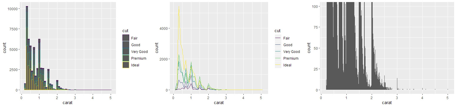
# Q1.变量怎么变化?
diamonds %>% count(cut) # 离散变量频数
diamonds %>% count(cut_width(carat, 0.5)) # 连续变量频数
e <- ggplot(diamonds, aes(x=carat)) # 定义绘图变量
e + geom_histogram(aes(color=cut), binwidth=0.1) # 堆叠直方图
e + geom_freqpoly(aes(color=cut), binwidth=0.1) # 分组密度图
e + geom_histogram(binwidth=0.01) + # 更精确的直方图
coord_cartesian(ylim = c(0,100)) # 放大y轴
# 从分布图可以看到存在较多离群值
diamonds %>% filter(between(y, 3, 20)) # 过滤离群值,删除整行
diamonds %>% mutate(y=ifelse(y<3|y>20, NA, y)) # 用缺失值代替离群值
diamonds %>% mutate(bool=is.na(y)) # 用新列标记缺失值
1
2
3
4
5
6
7
8
9
10
11
12
13
14
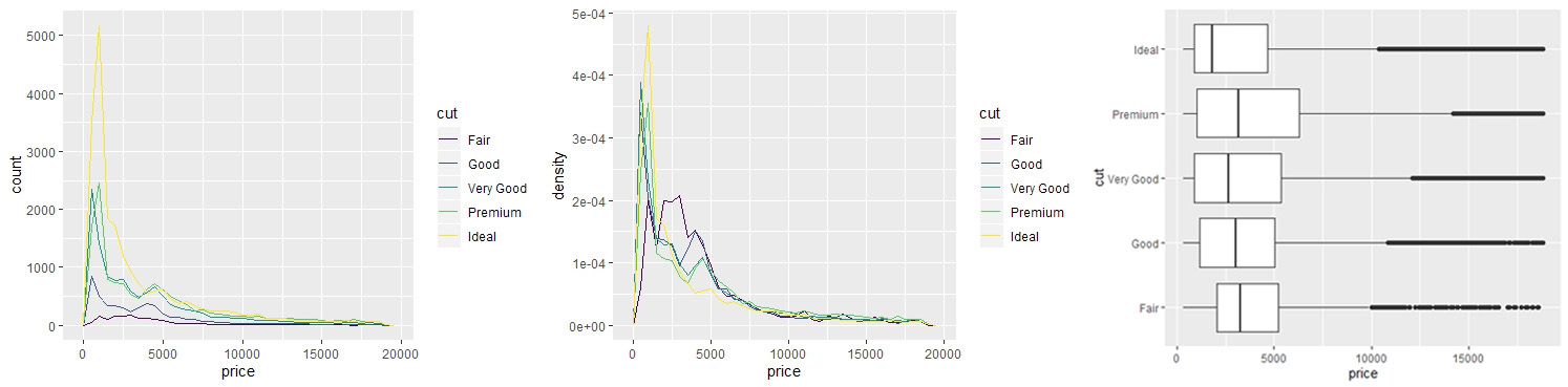
# Q2.变量之间的相关性?
# Q2-1.连续变量与离散变量的相关性
# 使用分组密度图
e <- ggplot(diamonds, aes(x=price))
# cut 与 price 的相关性
e + geom_freqpoly(aes(color=cut), binwidth=500)
# 使用y=..density..显示标准化的分布,易于比较
e + geom_freqpoly(aes(y=..density.., color=cut), binwidth=500)
# 用箱形图
e <- ggplot(diamonds, aes(x=cut, y=price))
e + geom_boxplot() + coord_flip()
1
2
3
4
5
6
7
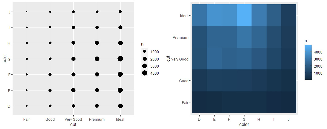
# Q2-2.离散变量与离散变量的相关性
# 点阵图
ggplot(diamonds) + geom_count(aes(x=cut, y=color))
# 热力图
diamonds %>% count(color, cut) %>%
ggplot(aes(x=color, y=cut)) + geom_tile(aes(fill=n))
1
2
3
4
5
6
7
8
9
10
11
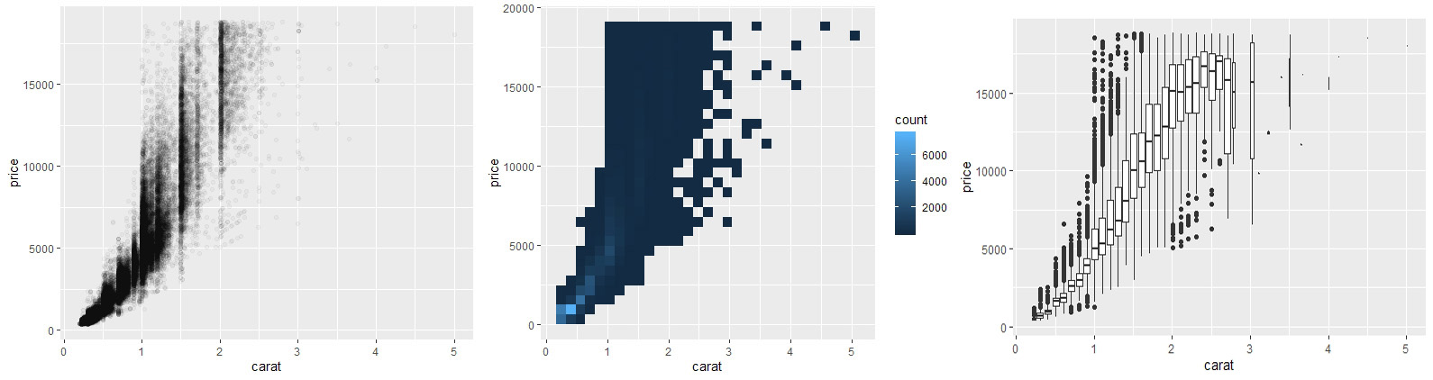
# Q2-3.连续变量与连续变量的相关性
e <- ggplot(diamonds, aes(x=carat, y=price))
# 散点图(用灰度表示频数密度)
e + geom_point(alpha=3/100)
# 网格图
e + geom_bin2d()
# 将其中一个变量离散化
e + geom_boxplot(aes(group=cut_width(carat, 0.1)))
CHPT06 - Workflow: Projects
- 不要依赖workspace保存环境,在代码里创造环境;
- 可以使用:
Ctrl+Shift+F10重启,然后用Ctrl+Shift+S重新运行 scripts 测试代码完整性; - 把所有的输入数据,脚本,分析结果,图像关联到一个project里面;
- 使用相对路径而不是绝对路径。
CHPT07 - Tibbles with tibble
数据处理的标准流程:
- Import
- Tidy
- EDA (transforming –> visualising –> modeling)
- Communicate(report, visualising for communication)
Tibble:data.frame 的优化版本,功能更强
1
2
3
4
5
6
7
8
9
10
11
12
13
14
15
16
# 创建 tibble 对象
tibble(x=1:5, y=1, z=x^2+y)
# 使用 tribble 函数创建
tribble(
    ~x, ~y, ~z,
    "A", 1, TRUE,
    "B", 2, FALSE
)
# 强制转换 data.frame 对象
as.tibble(iris)

# tibble 显示更整齐,显示数据类型,并且可以强制显示所有变量
nycflights13::flights %>% print(n=20, width=Inf)
# 索引方式
tb <- tibble(x=runif(10), y=rnorm(10))
tb$x; tb[["x"]]; tb[[1]]; tb $>$ .$x
CHPT08 - Import Data with readr
基本操作
1
2
3
4
5
6
7
data <- read.csv('C:/Users/Paradise/Desktop/test.csv')
data <- read_csv(
    "a, b, c
    1, 2, 3
    4, 5, 6", col_names=c('x', 'y', 'z')
)
# 使用 read_csv_chunked(file, chunk_size) 分块读取大文件
数据整理
1
2
3
4
5
6
7
8
9
10
11
12
13
14
15
16
17
18
# 统一数据类型
lst = c('1, 2, data$b, TRUE, TRUE, FALSE')
parse_integer(lst)
parse_logical(lst)

# 字符串 --> ASCII 编码
charToRaw("AaBbCc")
# 编码 --> 字符串
eco <- '\x82\xb1\x82\xf1\x82\xc9\x82\xbf\x82\xcd'
parse_character(eco, locale=locale(encoding='Shift-JIS'))
# 匹配字符串编码方式
guess_encoding(charToRaw("こんにちは"))

# 时间日期
parse_datetime('2020-10-01T123456')
parse_time('12:34 am')
parse_date("10/01/20","%m/%d/%y")
parse_date("1 October 2020","%d %B %Y")
CHPT09 - Tidy Data with tidyr
常见问题一:一个变量分布在多列
1
2
3
4
5
6
7
8
9
10
11
12
13
14
15
16
17
18
19
20
exmp1 <- read_csv(
    "country,   2017,   2018
    Asgard,     745,    2666
    Wakanda,    7737,   8048
    Titan,      2125,   2376"
)
# 使用 gather 函数整理:
tidy1 <- exmp1 %>% gather('2017', '2018', key='year', value='values')

--------------------------------
> tidy1
# A tibble: 6 x 3
  country year  values
  <chr>   <chr>  <dbl>
1 Asgard  2017     745
2 Wakanda 2017    7737
3 Titan   2017    2125
4 Asgard  2018    2666
5 Wakanda 2018    8048
6 Titan   2018    2376
常见问题二:一个观测分布在多行
1
2
3
4
5
6
7
8
9
10
11
12
13
14
15
16
17
18
19
20
21
22
23
exmp2 <- read_csv(
    "coutry,    year,   type,   values
    Asgard,     1999,   A,      745
    Asgard,     1999,   B,      18707
    Asgard,     2000,   A,      2666
    Asgard,     2000,   B,      59536
    Wakanda,    1999,   A,      7737
    Wakanda,    1999,   B,      30636
    Wakanda,    2000,   A,      8048
    Wakanda,    2000,   B,      50489"
)
# 使用 spread 函数整理(gather 的逆操作)
tidy2 <- exmp2 %>% spread(key='type', value='values')

---------------------------------
> tidy2
# A tibble: 4 x 4
  coutry   year     A     B
  <chr>   <dbl> <dbl> <dbl>
1 Asgard   1999   745 18707
2 Asgard   2000  2666 59536
3 Wakanda  1999  7737 30636
4 Wakanda  2000  8048 50489
常见问题三:一个列包含多个变量
1
2
3
4
5
6
7
8
9
10
11
12
13
14
15
16
17
exmp3 <- read_csv(
    "country,   year,   heros
    Asgard,     1999,   Thor/Loki
    Asgard,     2000,   Odin/Heimdall
    Midgard,    1999,   Hulk/BlackWidow"
)
# 使用 separate 分离两个变量(逆操作:unite)
tidy3 <- exmp3 %>% separate(heros, into=c('A', 'B'))

---------------------------------
> tidy3
# A tibble: 3 x 4
  country  year A     B
  <chr>   <dbl> <chr> <chr>
1 Asgard   1999 Thor  Loki
2 Asgard   2000 Odin  Heimdall
3 Midgard  1999 Hulk  BlackWidow
CHPT10 - Relational Data with dplyr
1
2
3
4
5
6
7
8
9
10
11
12
13
14
15
16
17
18
19
20
21
22
23
24
25
26
27
28
29
30
31
32
33
34
35
36
37
38
39
40
41
42
43
44
45
# 确定变量取值是否唯一
library(nycfights13)
planes %>% count(tailnum) %>% filter(n>1)

# 联结表
filghts %>% left_join(airlines, by='carrier')
# 使用 mutate 实现同等效果:
mutate(flights, name=airlines$name[match(carrier, airlines$carrier)])

# Inner/Outer Joins:
x<-tribble(
    ~key,   ~x,
    1,      "x1",
    2,      "x2",
    3,      "x3"
)
y<-tribble(
    ~key,   ~y,
    1,      "y1",
    2,      "y2",
    4,      "y4"
)
inner_join(x,y,by="key")    # 结果值保留key相同的部分(交集)
left_join(x,y,by="key")     # 第一个参数的key保全,第二个参数进行匹配
right_join(x,y,by="key")    # 与上一例相反
full_join(x,y,by="key")     # 全部key的值都保留

# 使用 merge 实现以上对应的操作
merge(x, y)
merge(x, y, all.x=T)
merge(x, y, all.y=T)
merge(x, y, all.x=T, all.y=T)

# Filtering Joins
top_dest <- filghts %>% count(dest, sort=T) %>% head(10)
flights %>% filter(dest %in% top_dest$dest)     # top 10 目的地
# 使用 semi_join 代替手动进行 filter
semi_join(flights, top_dest)
# 使用 anti_join 找出不匹配的部分
anti_join(flights, planes, by='tailnum')

# 集合操作
intersect(x, y)     # 交集
union(x, y)         # 与非
setdiff(x, y)       # x - y
CHPT11 - Strings with stringr
1
2
3
4
5
6
7
8
9
10
11
12
13
14
15
16
17
18
19
20
21
22
23
24
# 字符串操作
library(stringr)

# str_ 函数族
str_length('ABC')
str_c('(', c('b', 'c', 'd'), ')', sep='-')
# [1] "(-b-)" "(-c-)" "(-d-)"           # 支持向量化
str_c(if (TRUE) 'FUCK!')                # 支持条件语句
str_sub('abcde', 1, 3)                  # 取子集:1-3
str_to_lower('ABC')                     # 转为小写
str_view('abcd', 'a.*?')                # 使用正则表达式匹配
str_detect(c('ab', 'bc', 'cd'), '.b')   # 同上,返回布尔型
str_subset(c('ab', 'bc', 'cd'), 'b.')   # 同上,返回子集
str_subset(c('ab', 'bc', 'cd'), 'a')    # 同上,返回计数值
str_view_all(c('ab', 'bc', 'cd'), 'ab') # 同上,全字匹配
str_split('a,b,c,d,e', ',')             # 按特定字符切割

# str_replace
# 替换第一个找到的匹配
c('abc', '123') %>% str_replace('[bc23]', '-')
# 替换全部匹配值
c('abc', '123') %>% str_replace_all('[bc23]', '-')
# 替换为不同的值
c('abc', '123') %>% str_replace_all(c('a'='-', '1'='+'))
CHPT12 - Factors with forcats
1
2
3
4
5
6
7
8
9
10
11
12
13
14
# 处理因子变量
library(forcats)

# 使用 factor 对象:
# 直接使用 sort 按字母排序
x <- c("Dec", "Apr", "Jan", "Mar")
sort(x)
# 创建 levels
month_level <- c("Jan","Fed","Mar","Apr","May","Jun",
                 "Jul","Aug","Sep","Oct","Nov","Dec")
# 将 x 转化为带有 level 的离散变量
y <- factor(x, levels=month_level)
# 对 factor 对象使用 sort 按照 level 排序
sort(y)
CHPT13 - Dates and Times with lubridate
1
2
3
4
5
6
7
8
9
10
11
12
13
14
15
16
17
18
19
20
21
22
23
24
25
26
27
28
29
30
31
32
33
34
35
36
37
38
39
40
41
42
43
44
45
# 使用 lubridate 处理时间日期
library(lubridate)
library(nycflights13)

# 常用函数
today()
ymd('2020-10-19')
mdy('January 31st, 2020')
dmy('31-Jan-2020')
mdy_h('10192012')           # 2020-10-19 12:00:00 UTC
ymd_hms('201019 120000')
ymd(20201019, tz='UTC')     # 支持数值型,支持指定时区

# 操作示例
flights %>% select(year, month, day, hour, minute) %>%
    mutate(departure=make_datetime(year, month, day, hour, minute))

# 其他创建时间日期对象的形式
as_datetime(today())
as_date(now())
exmp <- ymd_hms('20201019 120001')
year(exmp)
wday(exmp, label=TRUE, abbr=FALSE)

# 修改时间日期对象
year(exmp) <- 2019
hour(exmp) <- hour(exmp) + 1
update(exmp, year=2019)

# 时间跨度对象 durations (秒格式)
age <- today() - ymd(19950825)
age <- as.duration(age)
aweek <- ddays(7)

# 时间跨度对象 Periods (年月日时分秒格式)
years(1)+months(2)+days(3)+hours(4)+minutes(5)+seconds(6)
# 用于计算时间推移
today() + years(1)

# 时区与本地化
Sys.timezone()      # 查看系统的时区
OlsonNames()        # 查看 R 支持的所有时区
t1 <- ymd_hms("20201020 000000", tz="America/New_York")
t2 <- ymd_hms("20201020 060000", tz="Europe/Copenhagen")
t1 - t2 == 0        #TRUE
CHPT14~15 Pipes & Functions
SKIP
CHPT16 - Vectors
基础知识
- 两类向量:
- 原子型向量:
- 整型、双整型、字符型、复数型、逻辑型、raw
- 列表:循环向量、列表中包含列表
- 原子型向量:
- NULL 与 NA:前者表示缺失的向量,后者表示确实的某个值
- 向量的两个关键性质:类型、长度
- 属性与增广矩阵:
- 整型向量的因子
- 数值型向量的时间日期
- 列表的数据框
示例
1
2
3
4
5
6
7
8
9
10
11
12
13
14
15
16
17
18
19
20
21
22
23
24
25
26
27
28
29
30
31
32
33
34
35
36
37
38
39
40
41
42
43
44
45
46
47
48
49
50
51
52
53
54
55
56
57
58
59
60
61
62
63
64
65
66
67
68
69
70
71
72
73
74
75
76
77
78
79
80
81
82
83
84
85
86
87
88
89
90
91
92
93
# (1)数值型 ----------------------------------------
typeof(1)       # double
class(1)        # numeric
typeof(1L)      # integer
class(1L)       # integer

# 整型(integer)和双整型(double)的区别:
# 所有双整型数据都是有限精度的浮点数
sqrt(2)^2 == 2              # FALSE
dplyr::near(sqrt(2)^2, 2)   # TRUE
# 双整型除了 NA 还有三类特殊值
c(-1, 0, 1) / 0             # -Inf NaN Inf
# 对应的判别函数:is.infinite() is.finite() is.nan()

# (2)字符型 ----------------------------------------
#重要特点:在R中字符型储存在全局环境,只储存一次,以减少空间占用
x <- "This is a really long string."
object.size(x)              #136 bytes
y <- rep(x, 1000)           #产生一个字符型向量
object.size(y)              #8128 bytes--一个指针8bytes,因此约为8000bytes

# (3)向量的强制转换 -----------------------------------
# 显式的强制转换:as.integer()、as.character()、as.double()、as.logical()
# 隐式的强制转换:
exmp <- 1:10
sum(exmp > 5)                   # logical --> integer
if (lenth(exmp)) {print('integer --> logical')}

# 强制转换的优先级
typeof(c(TRUE, 1L))             # integer
typeof(c(1L, 1.1))              # double
typeof(c(TRUE, 1L, 1.1, 'A'))   # character

# (4)向量化循环规则 ------------------------------------
1:10 + 1:3      # 2  4  6  5  7  9  8 10 12 11

# (5)向量取子集 ---------------------------------------
x <- c("one", "two", "three", "four", "five")
x[c(1, 3, 5)]
x[c(1, 1, 3, 3)]
x[c(-1, -3, -5)]        # 负值表示取其余集
x <- set_names(1:5,x)   # 命名
x["one"]                # 类型为 Named int,可以用名称进行索引

# (6)循环向量:列表 -------------------------------------
#列表可以包括列表,因此可以创建分层结构或树形结构
x_named <- list(a=c(1,2,3), b=c(4,5,6), c=c(7,8,9))
str(x_named)            #使用str函数打印列表
y <- list("a", 1.5, 1L, TRUE)
==============
> str(y)
List of 4
 $ : chr "a"
 $ : num 1.5
 $ : int 1
 $ : logi TRUE
==============

# (7)列表取子集 -----------------------------------------
exmp <- list(a=1:3, b="a string", c=pi, d=list(1,2))
exmp[1:2]
str(exmp[3])        # 返回向量
str(exmp[[3]])      # 返回数值
x_named[[3]]        # 返回数值向量7,8,9
x_named[[3]][1]     # 返回数值7
exmp$d              # 名称索引,等同于exmp[["d"]]

# (8)Attributes属性 ------------------------------------
x <- 1:10
attr(x, "greeting")
attr(x, "greeting") <- "hi"
attr(x, "farewell") <- "bye"
===============
> attributes(x)
$greeting
[1] "hi"
$farewell
[1] "bye"
===============
# 三种重要属性:names、dimensions、class;用于面相对象的S3系统
# S3系统:控制泛函的工作
# 泛函:输入的类不同函数的功能不同

# (9)增广向量 Augmented Vectors:带有附加属性的原子型向量 ----------
x <- factor(c("a","b","c"), levels=c("a","b","c","d"))
typeof(x)           # "interge"
===================
> attributes(x)
$`levels`
[1] "a" "b" "c" "d"
$class
[1] "factor"
===================
CHPT17 - 使用 purrr 进行迭代
1
2
3
4
5
6
7
8
9
10
11
12
13
14
15
16
17
18
19
20
21
22
23
24
25
26
27
28
29
30
31
32
33
34
35
36
37
38
39
40
41
42
43
44
45
46
47
48
49
50
51
52
53
54
55
56
57
58
59
60
61
62
63
64
65
library(tidyverse)
exmp <- tibble(a=rnorm(10), b=rnorm(10), c=rnorm(10), d=rnorm(10))

# 使用 for 循环计算每一行的中位数
output <- vector('double', ncol(exmp))
for (i in seq_along(exmp)) {
    output[i] <- median(exmp[[i]])
}

# 使用 map 代替 for 循环 ------------------------------------------------
output <- exmp %>% map(median)      # map 每一行
exmp %>% t(.) %>% map(median)       # map 每一列

# 在 map 中定义函数
# 按气缸数目cyl分成几部分,对每部分进行 mpg~wt 的线性回归
models <- mtcars %>% split(.$cyl) %>% map(
    function(exmp) lm(mpg~wt,data=exmp)
)

# 可以在map函数里面加入被引用函数的参数
mul <- list(3,7,-2)
mul %>% map(rnorm, n=5) %>% str()
# 如果还需要增加方差变量
sigma <- list(1,5,10)
seq_along(mul) %>% map(~rnorm(5, mul[[.]], sigma[[.]])) %>% str()

# 多个输入变量的map:map2()/pmap() ---------------------------------------

# 使用map2可以直接将map应用到两个向量,互不干扰
map2(mul, sigma, rnorm, n=5) %>% str()
# map2 算法:
map2inside<-function(x,y,f,...){        # 用省略号定义未知参数
  out<-vector("list",length(x))         # x与y的长度应相等
  for (i in seq_along(x)) {
    out[[i]]<-f(x[[i]],y[[i]],...)      # 向量化的操作
  }
  return(out)
}

# 当需要应用到多于两个的向量,可以使用pmap()
n<-list(1,3,5)
arg <- list(n,mul,sigma)
arg %>% pmap(rnorm) %>% str()
# 注意参数列表需要命名,并按照所引用函数的参数输入顺序
arg2 <- tribble(
    ~n,	~sd,~mean,
    1,	1,	3,
    3,	5,	7,
    5,	10,	-2
)
pmap(arg2, rnorm) %>% str()
#可以以数据框输入参数,参数不一定按顺序,但是要按照被引用函数的参数名称对参数变量进行命名

# 其他形式的for循环 ------------------------------------------------

# 谓语函数
keep(iris, is.factor) %>% str()     # 保留谓语返回TRUE时的部分,谓语指is.factor语句
discard(iris, is.factor) %>% str()  # 保留谓语返回FALSE时的部分
x <- list(1:5, letters, list(10))
some(x, is.character)               # 返回TRUE,翻译为:is some of x is character?
every(x, is.vector)                 # TRUE,翻译为:is every one of x is vector?
x <- sample(10)
detect(x, ~.>8)         # 返回第一个使得谓语为TRUE的内容
head_while(x,~.>5)      # 从头开始返回使得谓语为TRUE的内容
tail_while(x,~.>4)      # 从尾开始返回使得谓语为TRUE的内容