本文为笔记,原文链接:http://liyangbit.com/pythonvisualization/matplotlib-top-50-visualizations/
本文在代码 jupyter notebook 运行,在当前文件夹打开 cmd 执行:
jupyter nbconvert --to script *.ipynb可以把.ipynb文件保存为.py脚本文件。
环境准备
1
2
3
4
5
6
7
8
9
10
11
12
13
14
15
16
17
18
19
20
21
22
import numpy as np
import pandas as pd
import matplotlib as mpl
import matplotlib.pyplot as plt
import seaborn as sns
import warnings
warnings.filterwarnings(action='once')
"""
#绘图参数设置
large=22;med=16;small=12
params={'axes.titlesize':large,
        'legend.fontsize':med,
        'figure.figsize':(16,10),
        'axes.labelsize':med,
        'axes.titlesize':med,
        'xtick.labelsize':med,
        'ytick.labelsize':med,
        'figure.figsize':large}
plt.rcParams.update(params) """
plt.style.use('seaborn-whitegrid')
sns.set_style('white')
%matplotlib inline
1
2
3
#版本信息
print(mpl.__version__)
print(sns.__version__)
1
2
3.0.2
0.9.0
一、关联(Correlation)
散点图
1
2
3
4
midwest = pd.read_csv(
  "https://raw.githubusercontent.com/" +
  "selva86/datasets/master/midwest_filter.csv")
midwest.head()
| PID | county | state | area | poptotal | popdensity | popwhite | popblack | popamerindian | popasian | ... | percprof | poppovertyknown | percpovertyknown | percbelowpoverty | percchildbelowpovert | percadultpoverty | percelderlypoverty | inmetro | category | dot_size | |
|---|---|---|---|---|---|---|---|---|---|---|---|---|---|---|---|---|---|---|---|---|---|
| 0 | 561 | ADAMS | IL | 0.052 | 66090 | 1270.961540 | 63917 | 1702 | 98 | 249 | ... | 4.355859 | 63628 | 96.274777 | 13.151443 | 18.011717 | 11.009776 | 12.443812 | 0 | AAR | 250.944411 |
| 1 | 562 | ALEXANDER | IL | 0.014 | 10626 | 759.000000 | 7054 | 3496 | 19 | 48 | ... | 2.870315 | 10529 | 99.087145 | 32.244278 | 45.826514 | 27.385647 | 25.228976 | 0 | LHR | 185.781260 |
| 2 | 563 | BOND | IL | 0.022 | 14991 | 681.409091 | 14477 | 429 | 35 | 16 | ... | 4.488572 | 14235 | 94.956974 | 12.068844 | 14.036061 | 10.852090 | 12.697410 | 0 | AAR | 175.905385 |
| 3 | 564 | BOONE | IL | 0.017 | 30806 | 1812.117650 | 29344 | 127 | 46 | 150 | ... | 4.197800 | 30337 | 98.477569 | 7.209019 | 11.179536 | 5.536013 | 6.217047 | 1 | ALU | 319.823487 |
| 4 | 565 | BROWN | IL | 0.018 | 5836 | 324.222222 | 5264 | 547 | 14 | 5 | ... | 3.367680 | 4815 | 82.505140 | 13.520249 | 13.022889 | 11.143211 | 19.200000 | 0 | AAR | 130.442161 |
1
2
3
4
5
6
7
8
9
10
11
12
13
14
15
16
17
18
19
20
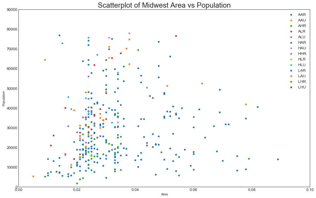
categories=np.unique(midwest['category'])
colors=[
plt.cm.tab10(i/float(len(categories)-1)) for i in range(len(categories))
]
plt.figure(figsize=(16,10), dpi=80, facecolor='w', edgecolor='K')
for i,category in enumerate(categories):
plt.scatter(
'area', 'poptotal',
data=midwest.loc[midwest.category==category,:],
s=20, cmap=colors[i], label=str(category)
)
plt.gca().set(
xlim=(0.0,0.1), ylim=(0,90000),
xlabel='Area', ylabel='Population')
plt.xticks(fontsize=12)
plt.yticks(fontsize=12)
plt.title("Scatterplot of Midwest Area vs Population",fontsize=22)
plt.legend(fontsize=12)
plt.show()
带边界的气泡图(Bubble plot with Encircling)
1
2
3
4
5
from matplotlib import patches
from scipy.spatial import ConvexHull
import warnings
warnings.simplefilter('ignore')
sns.set_style('white')
1
2
3
4
5
6
7
8
9
10
11
12
13
14
15
16
17
18
19
20
21
22
23
24
25
26
27
28
29
30
31
32
33
34
35
36
37
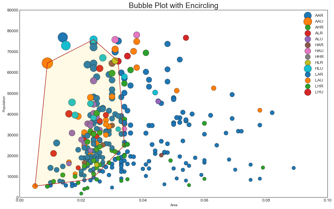
# Step 1: 数据准备,上一例散点图已经完成
# Step 2: Draw Scatterplot with unique color for each category
fig = plt.figure(figsize=(16, 10), dpi= 80, facecolor='w', edgecolor='k')
for i, category in enumerate(categories):
plt.scatter(
'area', 'poptotal',
data=midwest.loc[midwest.category==category, :],
s='dot_size', edgecolors='black',
cmap=colors[i], label=str(category), linewidths=.5)
# Step 3: Encircling
# https://stackoverflow.com/questions/44575681/
# how-do-i-encircle-different-data-sets-in-scatter-plot
def encircle(x,y, ax=None, **kw):
if not ax: ax=plt.gca()
p = np.c_[x,y]
hull = ConvexHull(p)
poly = plt.Polygon(p[hull.vertices,:], **kw)
ax.add_patch(poly)
# Select data to be encircled
midwest_encircle_data = midwest.loc[midwest.state=='IN', :]
# Draw polygon surrounding vertices
encircle(
midwest_encircle_data.area, midwest_encircle_data.poptotal,
ec="k", fc="gold", alpha=0.1)
encircle(
midwest_encircle_data.area, midwest_encircle_data.poptotal,
ec="firebrick", fc="none", linewidth=1.5)
# Step 4: Decorations
plt.gca().set(
xlim=(0.0, 0.1), ylim=(0, 90000), xlabel='Area', ylabel='Population')
plt.xticks(fontsize=12); plt.yticks(fontsize=12)
plt.title("Bubble Plot with Encircling", fontsize=22)
plt.legend(fontsize=12)
plt.show()
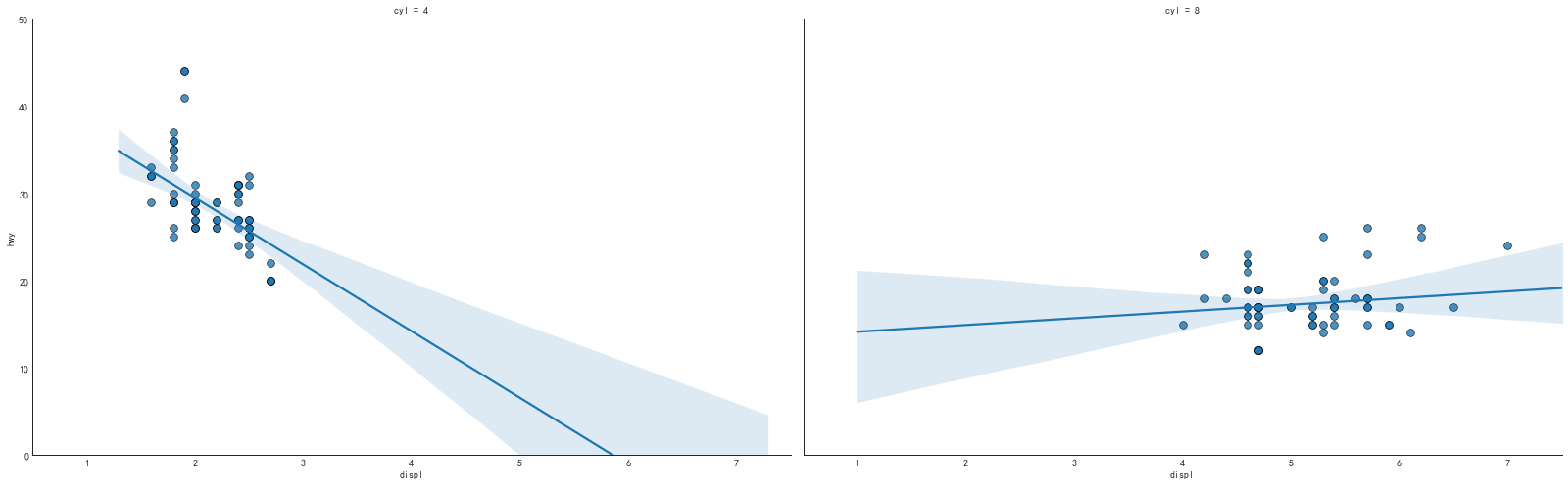
带线性回归最佳拟合点的散点图
1
2
3
4
5
#导入数据
df = pd.read_csv(
    "https://raw.githubusercontent.com/selva86/datasets/master/mpg_ggplot2.csv"
)
df.info()
1
2
3
4
5
6
7
8
9
10
11
12
13
14
15
16
    <class 'pandas.core.frame.DataFrame'>
    RangeIndex: 234 entries, 0 to 233
    Data columns (total 11 columns):
    manufacturer    234 non-null object
    model           234 non-null object
    displ           234 non-null float64
    year            234 non-null int64
    cyl             234 non-null int64
    trans           234 non-null object
    drv             234 non-null object
    cty             234 non-null int64
    hwy             234 non-null int64
    fl              234 non-null object
    class           234 non-null object
    dtypes: float64(1), int64(4), object(6)
    memory usage: 20.2+ KB
1
2
3
4
5
6
7
8
9
10
11
12
13
14
15
16
17
18
19
20
21
22
23
24
25
26
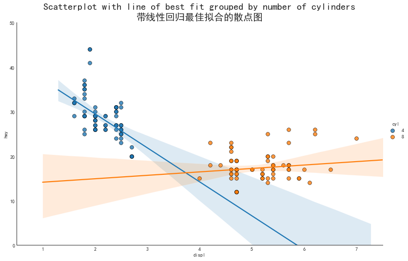
#数据预处理
df_select = df.loc[df.cyl.isin([4,8]), :]
print(df_select.head())
#绘图
sns.set_style("white")
#主要参数,x,y,分类变量hue,数据data
grid_obj = sns.lmplot(
x='displ', y='hwy', hue='cyl',
data=df_select,
height=7, aspect=1.6, robust=True, palette='tab10',
scatter_kws=dict(
s=60, linewidths=0.7, edgecolors='black'
)
)
#修饰图片
grid_obj.set(xlim=(0.5, 7.5), ylim=(0, 50))
#解决中文显示问题
plt.rcParams['font.sans-serif']=['SimHei']
plt.rcParams['axes.unicode_minus'] = False
#添加标题
plt.title(
"Scatterplot with line of best fit grouped by number of cylinders" +
"\n带线性回归最佳拟合的散点图",
fontsize=20)
plt.show()
1
2
3
4
5
6
7
8
9
10
#针对每类绘制带回归拟合的散点图(上图的拆分显示)
grid_obj = sns.lmplot(
    x='displ', y='hwy',col='cyl', data=df_select,
    height=7, aspect=1.6, robust=True, palette='Set1',
    scatter_kws=dict(s=60, linewidths=0.7, edgecolors='black')
    )
#主要修改了palette参数,以及把hue改为col参数
grid_obj.set(xlim=(0.5, 7.5), ylim=(0, 50))
#省略了修饰图片
plt.show()
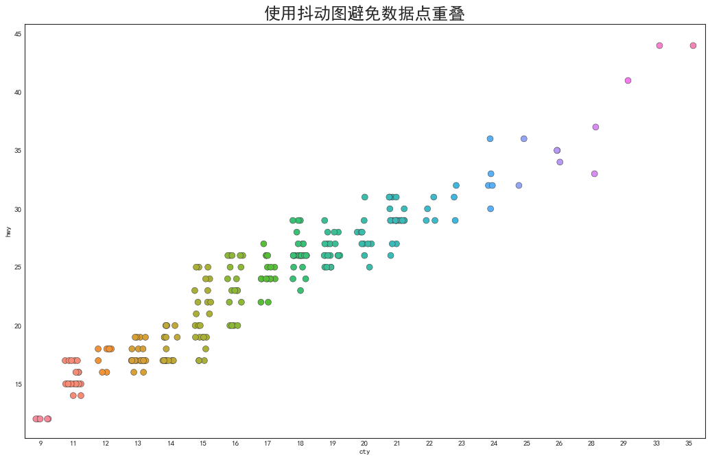
抖动图(Jittering with stripplot)
1
2
3
4
5
# 当多个数据点x和y值相等,绘图时会重叠,为了直观地看到所有数据点,使其稍微抖动
# 导入数据 >>
# https://raw.githubusercontent.com/selva86/datasets/master/mpg_ggplot2.csv
df = pd.read_csv("mpg_ggplot2.csv")  #直接读取网页csv报连接超时
print(df.head())
1
2
3
4
5
6
  manufacturer model  displ  year  cyl       trans drv  cty  hwy fl    class
0         audi    a4    1.8  1999    4    auto(l5)   f   18   29  p  compact
1         audi    a4    1.8  1999    4  manual(m5)   f   21   29  p  compact
2         audi    a4    2.0  2008    4  manual(m6)   f   20   31  p  compact
3         audi    a4    2.0  2008    4    auto(av)   f   21   30  p  compact
4         audi    a4    2.8  1999    6    auto(l5)   f   16   26  p  compact
1
2
3
4
5
6
7
#绘制抖动图
fig, ax = plt.subplots(figsize=(16,10), dpi=80)
sns.stripplot(df.cty, df.hwy, jitter=0.25, size=8, ax=ax, linewidth=0.5)
#先使用subplot得到图像对象和ax参数,在用stripplot完成绘图
#修饰图片
plt.title('使用抖动图避免数据点重叠', fontsize=22)
plt.show()
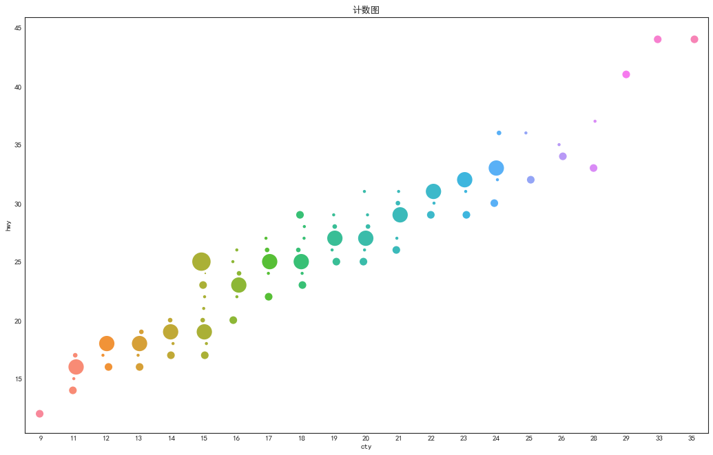
计数图(Counts Plot)
1
2
3
4
'''避免重叠的另一个方法是用点的大小表示重叠的点数量,体现某一点上的集中度'''
#导入数据
df = pd.read_csv('mpg_ggplot2.csv')
df.info()
1
2
3
4
5
6
7
8
9
10
11
12
13
14
15
16
<class 'pandas.core.frame.DataFrame'>
RangeIndex: 234 entries, 0 to 233
Data columns (total 11 columns):
manufacturer    234 non-null object
model           234 non-null object
displ           234 non-null float64
year            234 non-null int64
cyl             234 non-null int64
trans           234 non-null object
drv             234 non-null object
cty             234 non-null int64
hwy             234 non-null int64
fl              234 non-null object
class           234 non-null object
dtypes: float64(1), int64(4), object(6)
memory usage: 20.2+ KB
1
2
3
4
5
6
7
#数据准备:生成counts数据框
df_counts = df.groupby(['hwy', 'cty']).size().reset_index(name='counts')
#绘图:跟上例一样使用stripplot函数,但是改为使用size参数控制点的大小
fig, ax = plt.subplots(figsize=(16,10), dpi=80)
sns.stripplot(df_counts.cty, df_counts.hwy, size=df_counts.counts*2, ax=ax)
plt.title('计数图')
plt.show()
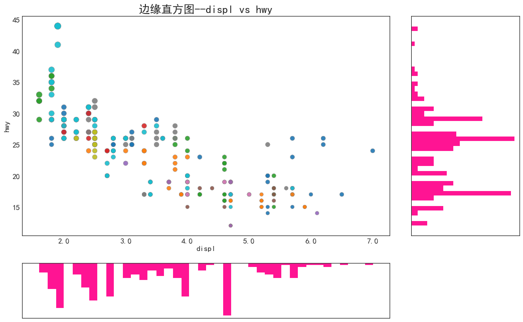
边缘直方图(Marginal Histogram)
1
2
3
4
5
6
7
8
9
10
11
12
13
14
15
16
17
18
19
20
21
22
23
24
25
26
27
28
29
30
31
32
33
34
35
36
37
38
39
40
41
'''沿X和Y轴变量的直方图'''
#导入数据
df = pd.read_csv('mpg_ggplot2.csv')
#创建图像和网格
fig = plt.figure(figsize=(16,10), dpi=80)
grid = plt.GridSpec(4, 4, hspace=0.5, wspace=0.2)
#定义axes
ax_main = fig.add_subplot(grid[:-1, :-1])
ax_right = fig.add_subplot(grid[:-1, -1], xticklabels=[], yticklabels=[])
ax_bottom = fig.add_subplot(grid[-1, 0:-1], xticklabels=[], yticklabels=[])

#main axe上画散点图
ax_main.scatter(
    'displ', 'hwy', data=df,
    c=df.manufacturer.astype('category').cat.codes,
    s=df.cty*4, alpha=0.9, cmap='tab10', edgecolors='gray', linewidths=0.5
)
#右方的直方图
ax_right.hist(
    df.hwy, 40, histtype='stepfilled', orientation='horizontal', color='orange'
)
#下方的直方图
ax_bottom.hist(
    df.displ, 40, histtype='stepfilled', orientation='vertical', color='orange'
)
ax_bottom.invert_yaxis()

#修饰图片
ax_main.set(title='边缘直方图--displ vs hwy', xlabel='displ', ylabel='hwy')
ax_main.title.set_fontsize(20)
for item in (
    [ax_main.xaxis.label, ax_main.yaxis.label] +
    ax_main.get_xticklabels() +
    ax_main.get_yticklabels()
    ):
    item.set_fontsize(14)

xlabels = ax_main.get_xticks().tolist()
ax_main.set_xticklabels(xlabels)

plt.show()
边缘箱形图(Marginal Boxplot)
1
2
3
4
5
6
7
8
9
10
11
12
13
14
15
16
17
18
19
20
21
22
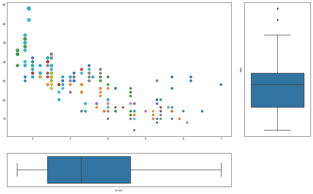
'''构建图片主要内容的过程与上图一样'''
df = pd.read_csv('mpg_ggplot2.csv')
#创建图像和网格
fig = plt.figure(figsize=(16,10), dpi=80)
grid = plt.GridSpec(4, 4, hspace=0.5, wspace=0.2)
#定义axes
ax_main = fig.add_subplot(grid[:-1, :-1])
ax_right = fig.add_subplot(grid[:-1, -1], xticklabels=[], yticklabels=[])
ax_bottom = fig.add_subplot(grid[-1, 0:-1], xticklabels=[], yticklabels=[])
#main axe上画散点图
ax_main.scatter(
'displ', 'hwy', data=df,
c=df.manufacturer.astype('category').cat.codes,
s=df.cty*4, alpha=0.9, cmap='tab10',edgecolors='gray',linewidths=0.5
)
#添加边缘箱形图
sns.boxplot(df.hwy, ax=ax_right, orient='v')
sns.boxplot(df.displ, ax=ax_bottom, orient='h')
#修饰图片与上图一样,略
plt.show()
相关图(Correlogram)
1
2
3
4
5
6
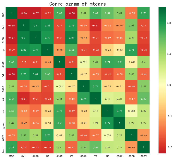
'''相关图用于直观地查看给定二维数组中所有的变量对之间的两两相关度量'''
#导入数据
df = pd.read_csv('https://github.com/selva86/datasets/raw/master/mtcars.csv')
print(df.head())
#两两相关系数:
print(df.corr())
1
2
3
4
5
6
7
8
9
10
11
12
13
14
15
16
17
18
19
20
21
22
23
24
25
26
27
28
29
30
31
32
33
34
35
36
37
38
39
40
        mpg  cyl   disp   hp  drat     wt   qsec  vs  am  gear  carb  fast  \
0  4.582576    6  160.0  110  3.90  2.620  16.46   0   1     4     4     1
1  4.582576    6  160.0  110  3.90  2.875  17.02   0   1     4     4     1
2  4.774935    4  108.0   93  3.85  2.320  18.61   1   1     4     1     1
3  4.626013    6  258.0  110  3.08  3.215  19.44   1   0     3     1     1
4  4.324350    8  360.0  175  3.15  3.440  17.02   0   0     3     2     1

                cars            carname
0          Mazda RX4          Mazda RX4
1      Mazda RX4 Wag      Mazda RX4 Wag
2         Datsun 710         Datsun 710
3     Hornet 4 Drive     Hornet 4 Drive
4  Hornet Sportabout  Hornet Sportabout
           mpg       cyl      disp        hp      drat        wt      qsec  \
mpg   1.000000 -0.858539 -0.867536 -0.787309  0.680312 -0.883453  0.420317
cyl  -0.858539  1.000000  0.902033  0.832447 -0.699938  0.782496 -0.591242
disp -0.867536  0.902033  1.000000  0.790949 -0.710214  0.887980 -0.433698
hp   -0.787309  0.832447  0.790949  1.000000 -0.448759  0.658748 -0.708223
drat  0.680312 -0.699938 -0.710214 -0.448759  1.000000 -0.712441  0.091205
wt   -0.883453  0.782496  0.887980  0.658748 -0.712441  1.000000 -0.174716
qsec  0.420317 -0.591242 -0.433698 -0.708223  0.091205 -0.174716  1.000000
vs    0.669260 -0.810812 -0.710416 -0.723097  0.440278 -0.554916  0.744535
am    0.593153 -0.522607 -0.591227 -0.243204  0.712711 -0.692495 -0.229861
gear  0.487226 -0.492687 -0.555569 -0.125704  0.699610 -0.583287 -0.212682
carb -0.553703  0.526988  0.394977  0.749812 -0.090790  0.427606 -0.656249
fast  0.730748 -0.695182 -0.732073 -0.751422  0.400430 -0.611265  0.488649

            vs        am      gear      carb      fast
mpg   0.669260  0.593153  0.487226 -0.553703  0.730748
cyl  -0.810812 -0.522607 -0.492687  0.526988 -0.695182
disp -0.710416 -0.591227 -0.555569  0.394977 -0.732073
hp   -0.723097 -0.243204 -0.125704  0.749812 -0.751422
drat  0.440278  0.712711  0.699610 -0.090790  0.400430
wt   -0.554916 -0.692495 -0.583287  0.427606 -0.611265
qsec  0.744535 -0.229861 -0.212682 -0.656249  0.488649
vs    1.000000  0.168345  0.206023 -0.569607  0.594588
am    0.168345  1.000000  0.794059  0.057534  0.283129
gear  0.206023  0.794059  1.000000  0.274073  0.266919
carb -0.569607  0.057534  0.274073  1.000000 -0.461196
fast  0.594588  0.283129  0.266919 -0.461196  1.000000
1
2
3
4
5
6
7
8
9
10
11
12
#绘图
plt.figure(figsize=(12,10), dpi=80)
sns.heatmap(
    df.corr(),
    xticklabels=df.corr().columns, yticklabels=df.corr().columns,
    cmap='RdYlGn', center=0, annot=True
)
#修饰图片
plt.title('Correlogram of mtcars', fontsize=20)
plt.xticks(fontsize=12)
plt.yticks(fontsize=12)
plt.show()
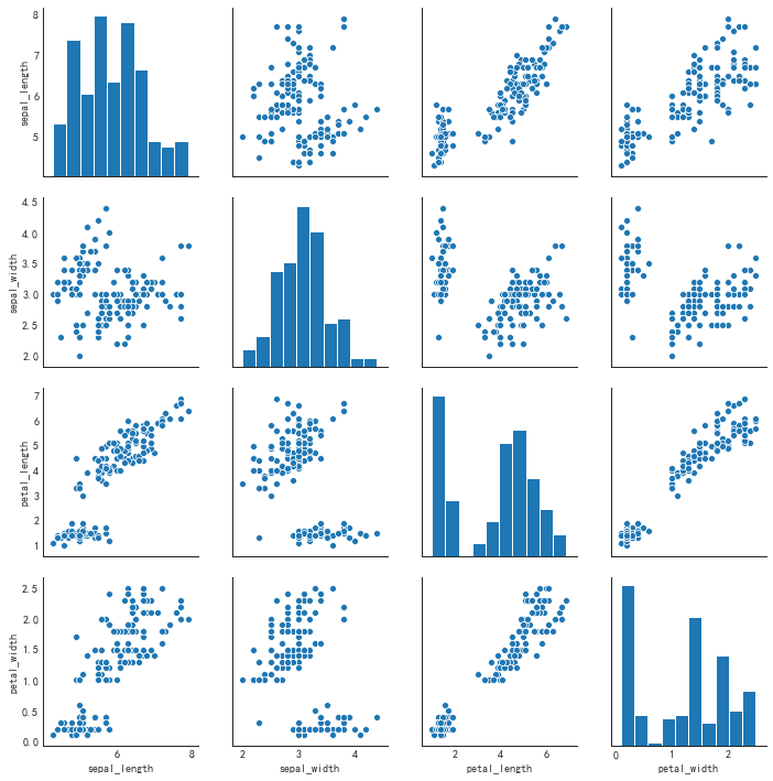
矩阵图(Pairwise Plot)
1
2
3
4
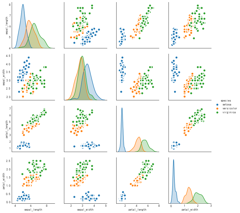
'''双变量分析常用绘图,给出两两的关联图,相当于R中的pairs函数'''
#导入数据
df = sns.load_dataset('iris')
df.info()
1
2
3
4
5
6
7
8
9
10
<class 'pandas.core.frame.DataFrame'>
RangeIndex: 150 entries, 0 to 149
Data columns (total 5 columns):
sepal_length    150 non-null float64
sepal_width     150 non-null float64
petal_length    150 non-null float64
petal_width     150 non-null float64
species         150 non-null object
dtypes: float64(4), object(1)
memory usage: 5.9+ KB
1
2
3
4
5
#绘图
plt.figure(figsize=(10,8), dpi=80)
sns.pairplot(df, kind='scatter', hue='species',#可以加入分类变量
             plot_kws=dict(s=80, edgecolor='white', linewidth=2.5))
plt.show()
1
2
3
4
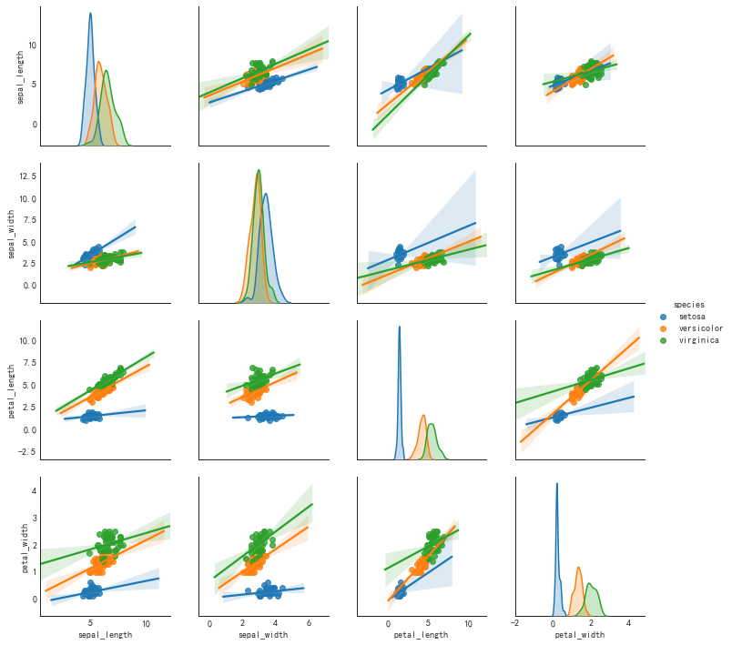
#图例2
plt.figure(figsize=(10,8), dpi=80)
sns.pairplot(df, kind='reg', hue='species')
plt.show()
1
2
#默认参数设置
sns.pairplot(df)
二、偏差(Deviation)
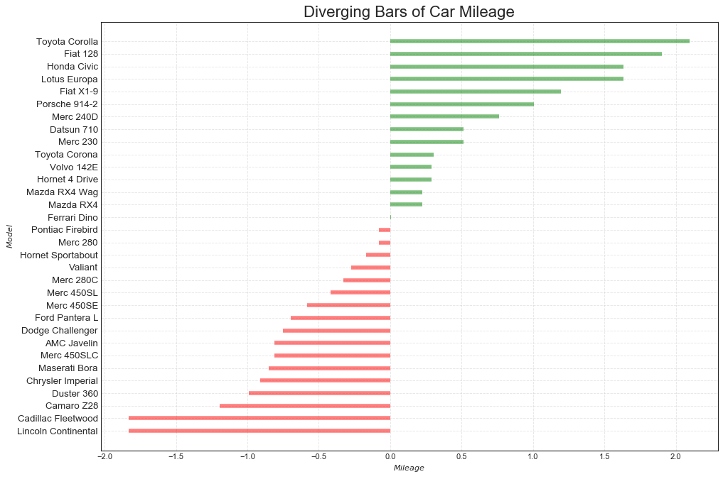
发散条形图(Diverging Bars)
1
2
3
4
5
6
7
8
9
10
11
12
13
14
15
'''可以根据单个指标查看项目的变化情况,并可视化此差异的顺序和数量'''
#导入数据
df = pd.read_csv('mtcars.csv')
#数据准备
# 抽取一列
x = df.loc[:, ['mpg']]
# 计算每个数据点相对于标准差的离散程度
df['mpg_z'] = (x - x.mean())/x.std()
# 分配颜色,增加颜色变量
df['colors'] = ['red' if i<0 else 'green' for i in df['mpg_z']]
# 按计算所得的 离散程度 重排数据
df.sort_values('mpg_z', inplace=True)
# 重排后 更新index
df.reset_index(inplace=True)
print(df.head())
1
2
3
4
5
6
7
8
9
10
11
12
13
   index       mpg  cyl   disp   hp  drat     wt   qsec  vs  am  gear  carb  \
0     15  3.224903    8  460.0  215  3.00  5.424  17.82   0   0     3     4
1     14  3.224903    8  472.0  205  2.93  5.250  17.98   0   0     3     4
2     23  3.646917    8  350.0  245  3.73  3.840  15.41   0   0     3     4
3      6  3.781534    8  360.0  245  3.21  3.570  15.84   0   0     3     4
4     16  3.834058    8  440.0  230  3.23  5.345  17.42   0   0     3     4

   fast                 cars              carname     mpg_z colors
0     0  Lincoln Continental  Lincoln Continental -1.829979    red
1     0   Cadillac Fleetwood   Cadillac Fleetwood -1.829979    red
2     0           Camaro Z28           Camaro Z28 -1.191664    red
3     0           Duster 360           Duster 360 -0.988049    red
4     0    Chrysler Imperial    Chrysler Imperial -0.908604    red
1
2
3
4
5
6
7
8
9
10
11
12
13
#绘图
plt.figure(figsize=(14,10), dpi=80)
plt.hlines(
    y=df.index,
    xmin=0, xmax=df.mpg_z, color=df.colors, alpha=0.5, linewidth=5
)
#主要参数:数据y,bar的长度xmin和xmax,colors,等
#修饰图片
plt.gca().set(ylabel='$Model$', xlabel='$Mileage$') # $号代表外层的新一级的标签
plt.yticks(df.index, df.cars, fontsize=12)
plt.title('Diverging Bars of Car Mileage', fontdict={'size':20}) # 使用字典的写法
plt.grid(linestyle='--', alpha=0.5)
plt.show()
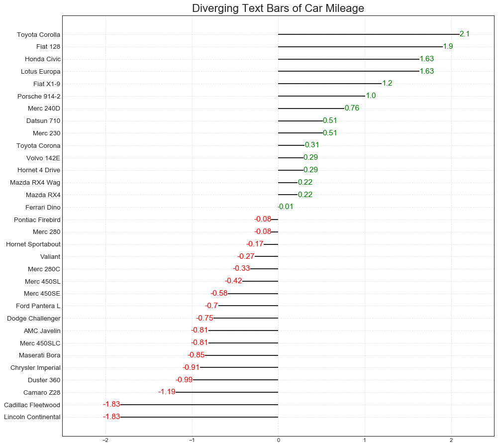
发散文本(Diverging Texts)
1
2
3
4
5
6
7
8
9
10
11
12
13
14
15
16
17
18
'''与上图类似,另外可以在图中加入文本强调一些内容'''
#数据准备与上例相同,直接绘图:
plt.figure(figsize=(14,14), dpi=80)
plt.hlines(y=df.index, xmin=0, xmax=df.mpg_z)
#增加文本
for x, y, tex in zip(df.mpg_z, df.index, df.mpg_z):
    t = plt.text(
        x, y, round(tex, 2),
        horizontalalignment='right' if x<0 else 'left',
        verticalalignment='center',
        fontdict={'color': 'red' if x<0 else 'green', 'size': 14}
    )
#修饰图片
plt.yticks(df.index, df.cars, fontsize=12)
plt.title('Diverging Text Bars of Car Mileage', fontsize=20)
plt.grid(linestyle='--', alpha=0.5)
plt.xlim(-2.5, 2.5)
plt.show()
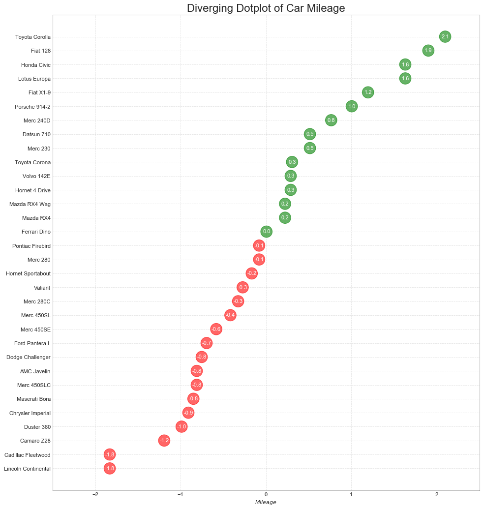
发散包点图(Diverging Dot Plot)
1
2
3
4
5
6
7
8
9
10
11
12
13
14
15
16
17
18
19
#数据准备同上,直接绘图
plt.figure(figsize=(14,16), dpi=80)
plt.scatter(df.mpg_z, df.index, s=450, alpha=0.6, color=df.colors)
for x, y, tex in zip(df.mpg_z, df.index, df.mpg_z):
    t = plt.text(x, y, round(tex, 1), horizontalalignment='center',
                verticalalignment='center', fontdict={'color': 'white'})

#修饰图片
plt.gca().spines['top'].set_alpha(0.3)
plt.gca().spines['bottom'].set_alpha(0.3)
plt.gca().spines['right'].set_alpha(0.3)
plt.gca().spines['left'].set_alpha(0.3)

plt.yticks(df.index, df.cars)
plt.title('Diverging Dotplot of Car Mileage', fontsize=20)
plt.xlabel('$Mileage$')
plt.grid(linestyle='--', alpha=0.5)
plt.xlim(-2.5, 2.5)
plt.show()
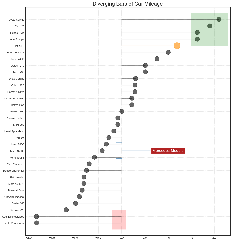
带标记的发散棒棒糖图(Diverging Lollipop Chart with Markers)
1
2
3
4
5
6
7
8
9
10
#数据准备
df = pd.read_csv('mtcars.csv')
x = df.loc[:, ['mpg']]
df['mpg_z'] = (x - x.mean())/x.std()
df['colors'] = 'black'

df.loc[df.cars == 'Fiat X1-9', 'colors'] = 'dackorange'
df.sort_values('mpg_z', inplace=True)
df.reset_index(inplace=True)
df.head()
| index | mpg | cyl | disp | hp | drat | wt | qsec | vs | am | gear | carb | fast | cars | carname | mpg_z | colors | |
|---|---|---|---|---|---|---|---|---|---|---|---|---|---|---|---|---|---|
| 0 | 15 | 3.224903 | 8 | 460.0 | 215 | 3.00 | 5.424 | 17.82 | 0 | 0 | 3 | 4 | 0 | Lincoln Continental | Lincoln Continental | -1.829979 | black |
| 1 | 14 | 3.224903 | 8 | 472.0 | 205 | 2.93 | 5.250 | 17.98 | 0 | 0 | 3 | 4 | 0 | Cadillac Fleetwood | Cadillac Fleetwood | -1.829979 | black |
| 2 | 23 | 3.646917 | 8 | 350.0 | 245 | 3.73 | 3.840 | 15.41 | 0 | 0 | 3 | 4 | 0 | Camaro Z28 | Camaro Z28 | -1.191664 | black |
| 3 | 6 | 3.781534 | 8 | 360.0 | 245 | 3.21 | 3.570 | 15.84 | 0 | 0 | 3 | 4 | 0 | Duster 360 | Duster 360 | -0.988049 | black |
| 4 | 16 | 3.834058 | 8 | 440.0 | 230 | 3.23 | 5.345 | 17.42 | 0 | 0 | 3 | 4 | 0 | Chrysler Imperial | Chrysler Imperial | -0.908604 | black |
1
2
3
4
5
6
7
8
9
10
11
12
13
14
15
16
17
18
19
20
21
22
23
24
25
26
27
28
29
30
31
32
33
34
35
36
37
38
#绘图
plt.figure(figsize=(14,16), dpi=80)
plt.hlines(
    y=df.index, xmin=0, xmax=df.mpg_z, color=df.colors, alpha=0.4, linewidth=1
)
plt.scatter(
    df.mpg_z, df.index, color=df.colors, alpha=0.6,
    s=[600 if x == 'Fiat X1-9' else 300 for x in df.cars]
)
plt.yticks(df.index, df.cars)
plt.xticks(fontsize=12)

#添加注释
plt.annotate(
    'Mercedes Models', xy=(0.0, 11.0), xytext=(1.0, 11),
    xycoords='data',
    fontsize=15, color='white', ha='center', va='center',
    bbox=dict(boxstyle='square', fc='firebrick'),
    arrowprops=dict(
        arrowstyle='-[, widthB=2.0, lengthB=1.5', lw=2.0, color='steelblue'
    ),
)

#添加补丁(框框)
from matplotlib import patches
p1 = patches.Rectangle(
    (-0.2, -1), width=0.3, height=3, alpha=0.2, facecolor='red'
)
p2 = patches.Rectangle(
    (1.5, 27), width=.8, height=5, alpha=0.2, facecolor='green'
)
plt.gca().add_patch(p1)
plt.gca().add_patch(p2)

#修饰图片
plt.title('Diverging Bars of Car Mileage', fontsize=20)
plt.grid(linestyle='--', alpha=0.5)
plt.show()
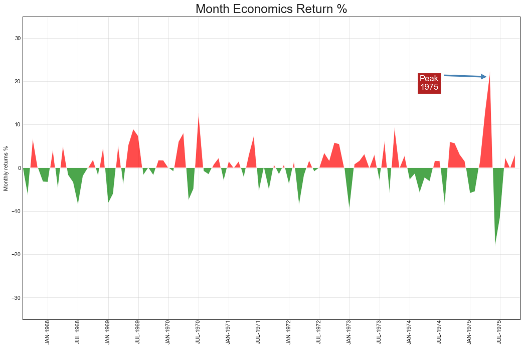
面积图(Area Chart)
1
2
3
4
5
6
'''通过填充颜色,面积图不仅强调峰和谷,还强调了其累积效应'''
#数据准备
df = pd.read_csv('economics.csv', parse_dates=['date']).head(100)
x = np.arange(df.shape[0])
y_returns = (df.psavert.diff().fillna(0)/df.psavert.shift(1)).fillna(0)*100
df.head()
| date | pce | pop | psavert | uempmed | unemploy | |
|---|---|---|---|---|---|---|
| 0 | 1967-07-01 | 507.4 | 198712 | 12.5 | 4.5 | 2944 |
| 1 | 1967-08-01 | 510.5 | 198911 | 12.5 | 4.7 | 2945 |
| 2 | 1967-09-01 | 516.3 | 199113 | 11.7 | 4.6 | 2958 |
| 3 | 1967-10-01 | 512.9 | 199311 | 12.5 | 4.9 | 3143 |
| 4 | 1967-11-01 | 518.1 | 199498 | 12.5 | 4.7 | 3066 |
1
2
3
4
5
6
7
8
9
10
11
12
13
14
15
16
17
18
19
20
21
22
23
24
25
26
27
28
29
30
31
32
33
34
35
#绘图
plt.figure(figsize=(16,10), dpi=80)
plt.fill_between(
    x[1:], y_returns[1:], 0, where=y_returns[1:] >= 0,
    facecolor='red', alpha=0.7, interpolate=True
)
plt.fill_between(
    x[1:], y_returns[1:], 0, where=y_returns[1:] <= 0,
    facecolor='green', alpha=0.7, interpolate=True
)

#添加注释
plt.annotate(
    'Peak\n1975', xy=(94,21), xytext=(80,18), fontsize=15, color='white',
    bbox={'boxstyle': 'square', 'fc': 'firebrick'},
    arrowprops={'facecolor': 'steelblue', 'shrink': 0.05}
)

#修饰图片
xtickvals = [
    str(m)[:3].upper() + '-'+str(y) for y,m in \
    zip(df.date.dt.year, df.date.dt.month_name())
]
plt.gca().set_xticks(x[::6])
plt.gca().set_xticklabels(
    xtickvals[::6], rotation=90,
    fontdict={
        'horizontalalignment':'center', 'verticalalignment':'center_baseline'
    }
)
plt.ylim(-35, 35), plt.xlim(1, 100)
plt.title("Month Economics Return %", fontsize=22)
plt.ylabel("Monthly returns %")
plt.grid(alpha=0.5)
plt.show()
三、排序(ranking)
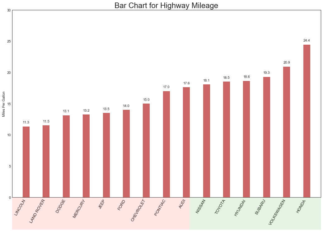
有序条形图
1
2
3
4
5
6
7
8
'''传达项目的排序信息,并可以添加度量值以提供更精确的信息'''
#数据准备
df_raw = pd.read_csv('mpg_ggplot2.csv')
#抽取两列,进行排序,并按照排序求均值
df = df_raw[['cty', 'manufacturer']].groupby('manufacturer').mean()
df.sort_values('cty', inplace=True)
df.reset_index(inplace=True)
print(df.head())
1
2
3
4
5
6
  manufacturer        cty
0      lincoln  11.333333
1   land rover  11.500000
2        dodge  13.135135
3      mercury  13.250000
4         jeep  13.500000
1
2
3
4
5
6
7
8
9
10
11
12
13
14
15
16
17
18
19
20
21
22
23
24
25
26
27
28
from matplotlib import patches
#绘图
fig, ax = plt.subplots(figsize=(16,10), facecolor='white', dpi=80)
ax.vlines(
    x=df.index, ymin=0, ymax=df.cty, color='firebrick', alpha=0.7, linewidth=20
)
#添加注释
for i, cty in enumerate(df.cty):
    ax.text(i, cty+0.5, round(cty, 1), horizontalalignment='center')
#修饰图片
ax.set_title('Bar Chart for Highway Mileage', fontsize=22)
ax.set(ylabel='Miles Per Gallon', ylim=(0,30))
plt.xticks(
    df.index, df.manufacturer.str.upper(),
    rotation=60, fontsize=12, horizontalalignment='right'
)
#添加补丁
p1 = patches.Rectangle(
    (0.57, -0.005), width=0.33, height=0.13, alpha=0.1,
    facecolor='green', transform=fig.transFigure
)
p2 = patches.Rectangle(
    (0.124, -0.005), width=0.446, height=0.13, alpha=0.1,
    facecolor='red', transform=fig.transFigure
)
fig.add_artist(p1)
fig.add_artist(p2)
fig.show()
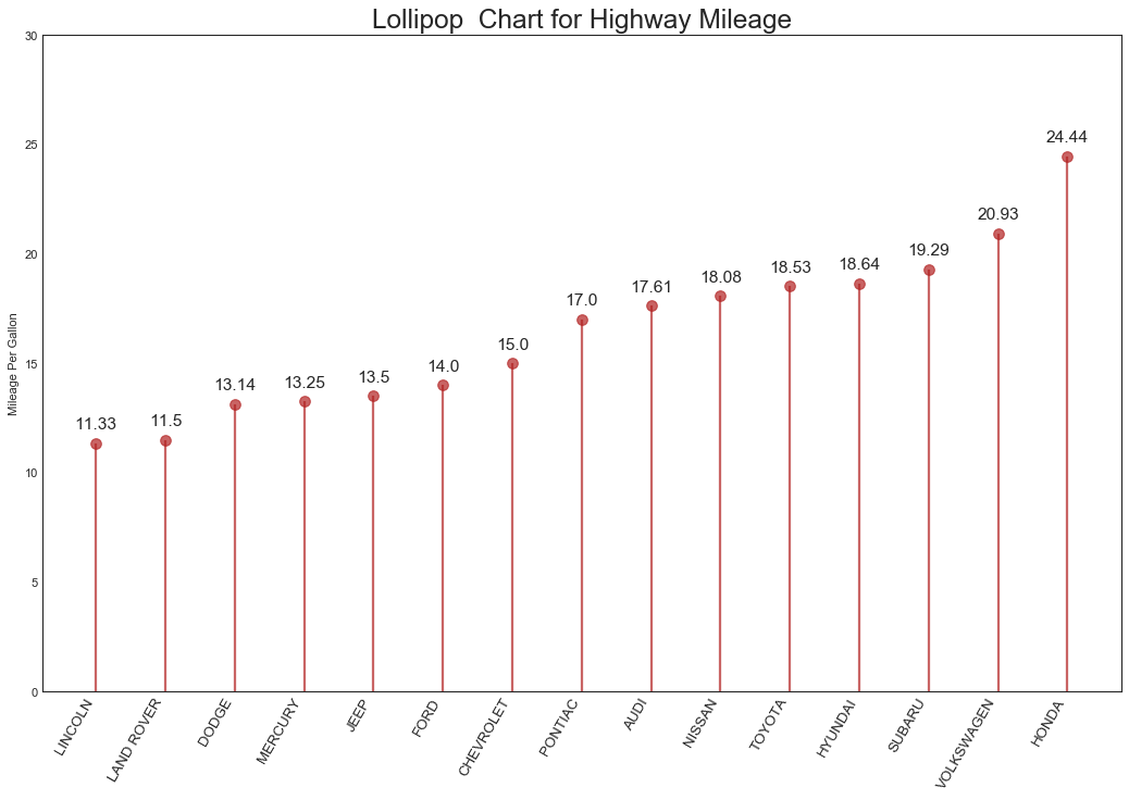
棒棒糖图
1
2
3
4
5
6
7
8
9
10
11
12
13
14
15
16
17
18
19
20
21
22
23
'''与有序条形图内容类似,风格更好看'''
#数据准备同上,绘图
fig, ax = plt.subplots(figsize=(16,10), dpi=80)
ax.vlines(
    x=df.index, ymin=0, ymax=df.cty, color='firebrick', alpha=0.7, linewidth=2
)
ax.scatter(x=df.index, y=df.cty, s=75, color='firebrick', alpha=0.7)
#修饰图片
ax.set_title('Lollipop  Chart for Highway Mileage', fontsize=22)
ax.set_ylabel('Mileage Per Gallon')
ax.set_xticks(df.index)
ax.set_xticklabels(
    df.manufacturer.str.upper(), rotation=60,
    fontdict={'horizontalalignment': 'right', "size": 12}
)
ax.set_ylim(0, 30)
#添加注释
for row in df.itertuples():
    ax.text(
        row.Index, row.cty+0.5, s=round(row.cty, 2),
        horizontalalignment='center', verticalalignment='bottom', fontsize=14
    )
plt.show()
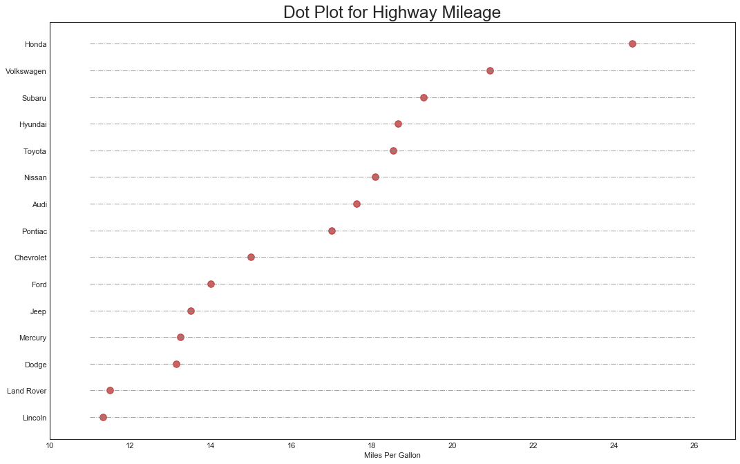
包点图(Dot Plot)
1
2
3
4
5
6
7
8
9
10
11
12
13
14
15
16
#数据准备同上,绘图
fig, ax = plt.subplots(figsize=(16,10), dpi=80)
ax.hlines(
    y=df.index, xmin=11, xmax=26,
    color='gray', alpha=0.7, linewidth=1, linestyles='dashdot'
)
ax.scatter(y=df.index, x=df.cty, s=75, color='firebrick', alpha=0.7)
#图片修饰
ax.set_title('Dot Plot for Highway Mileage', fontsize=22)
ax.set_xlabel('Miles Per Gallon')
ax.set_yticks(df.index)
ax.set_yticklabels(
    df.manufacturer.str.title(), fontdict={'horizontalalignment': 'right'}
)
ax.set_xlim(10, 27)
plt.show()
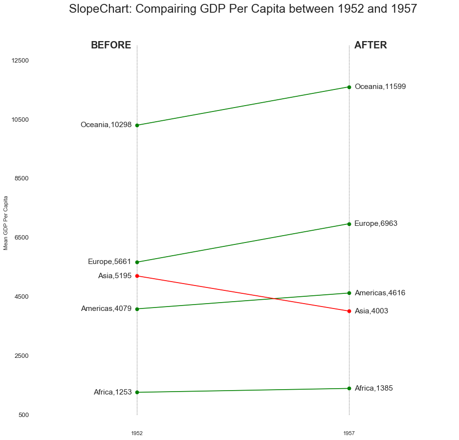
坡度图(Slope Chart)
1
2
3
4
5
6
7
8
9
10
11
12
13
'''坡度图适合用来比较给定项目的前后位置'''
from matplotlib import lines
#数据准备
df = pd.read_csv('gdppercap.csv')
left_label = [
    str(c) + ',' + str(round(y)) for c, y in zip(df.continent, df['1952'])
]
right_label = [
    str(c) + ',' + str(round(y)) for c, y in zip(df.continent, df['1957'])
]
klass = [
    'red' if (y1-y2) < 0 else 'green' for y1, y2 in zip(df['1952'], df['1957'])
]
1
2
3
4
5
6
7
8
9
10
#定义函数draw line
def newline(p1, p2, color='black'):
    ax = plt.gca()
    line = lines.Line2D(
        [p1[0], p2[0]], [p1[1], p2[1]],
        marker='o', markersize=6,
        color='red' if p1[1] - p2[1] > 0 else 'green'
    )
    ax.add_line(line)
    return line
1
2
3
4
5
6
7
8
9
10
11
12
13
14
15
16
17
18
19
20
21
22
23
24
25
26
27
28
29
30
31
32
33
34
35
36
37
38
39
40
41
42
43
44
45
46
47
48
49
50
51
52
53
54
55
56
57
#绘图
fig, ax = plt.subplots(1, 1, figsize=(14,14), dpi=80)
#画垂线
ax.vlines(
    x=1, ymin=500, ymax=13000,
    color='black', alpha=0.7, linewidth=1, linestyles='dotted'
)
ax.vlines(
    x=3, ymin=500, ymax=13000,
    color='black', alpha=0.7, linewidth=1, linestyles='dotted'
)
#散点
ax.scatter(
    y=df['1952'], x=np.repeat(1, df.shape[0]),
    s=10, color='black', alpha=0.7
)
ax.scatter(
    y=df['1957'], x=np.repeat(3, df.shape[0]),
    s=10, color='black', alpha=0.7
)
#注释
for p1, p2, c in zip(df['1952'], df['1957'], df['continent']):
    newline([1, p1], [3, p2])
    ax.text(
        1 - 0.05, p1, c + ',' + str(round(p1)),
        fontsize=14, horizontalalignment='right', verticalalignment='center'
    )
    ax.text(
        3 + 0.05, p2, c + ',' + str(round(p2)),
        fontsize=14, horizontalalignment='left', verticalalignment='center'
    )
#前后的注释
ax.text(
    1 - 0.05, 13000, 'BEFORE',
    fontdict={'size': 18, 'weight': 700},
    horizontalalignment='right', verticalalignment='center'
)
ax.text(
    3 + 0.05, 13000, 'AFTER',
    fontdict={'size': 18, 'weight': 700},
    horizontalalignment='left', verticalalignment='center'
)
#修饰图片
ax.set_title(
    "SlopeChart: Compairing GDP Per Capita between 1952 and 1957",
    fontsize=22
)
ax.set(xlim=(0,4), ylim=(0,14000), ylabel='Mean GDP Per Capita')
ax.set_xticks([1,3])
ax.set_xticklabels(['1952', '1957'])
plt.yticks(np.arange(500, 13000, 2000), fontsize=12)
#高亮边界
plt.gca().spines['top'].set_alpha(0)
plt.gca().spines['bottom'].set_alpha(0)
plt.gca().spines['right'].set_alpha(0)
plt.gca().spines['left'].set_alpha(0)
plt.show()
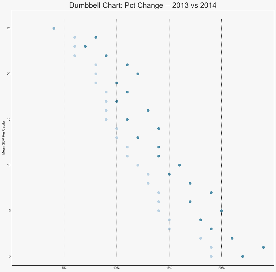
哑铃图(Dumbbell Plot)
1
2
3
4
5
6
"""哑铃图传达了各个项目的前后位置,以及项目的等级排序"""
from matplotlib import lines
#准备数据
df = pd.read_csv('health.csv')
df.sort_values('pct_2014', inplace=True)
df.reset_index(inplace=True)
1
2
3
4
5
6
#定义函数(类似上例)
def newline(p1, p2, color='black'):
    ax = plt.gca()
    line = mlines.Line2D([p1[0],p2[0]], [p1[1],p2[1]], color='skyblue')
    ax.add_line(line)
    return line
1
2
3
4
5
6
7
8
9
10
11
12
13
14
15
16
17
18
19
20
21
#绘图
fig, ax = plt.subplots(1, 1, figsize=(14,14), facecolor='#f7f7f7', dpi=80)
#垂线部分
ax.vlines(x=0.05, ymin=0, ymax=26, color='black', alpha=1, linewidth=1,
          linestyle='dotted')
ax.vlines(x=0.10, ymin=0, ymax=26, color='black', alpha=1, linewidth=1,
          linestyle='dotted')
ax.vlines(x=0.15, ymin=0, ymax=26, color='black', alpha=1, linewidth=1,
          linestyle='dotted')
ax.vlines(x=0.20, ymin=0, ymax=26, color='black', alpha=1, linewidth=1,
          linestyle='dotted')
#散点部分
ax.scatter(y=df['index'], x=df['pct_2013'], s=50, color='#0e668b', alpha=0.7)
ax.scatter(y=df['index'], x=df['pct_2014'], s=50, color='#a3c4dc', alpha=0.7)
#修饰图片
ax.set_facecolor('#f7f7f7')
ax.set_title("Dumbbell Chart: Pct Change -- 2013 vs 2014", fontsize=22)
ax.set(xlim=(0,0.25), ylim=(-1,27), ylabel='Mean GDP Per Capita')
ax.set_xticks([0.05, 0.10, 0.15, 0.20])
ax.set_xticklabels(['5%', '10%', '15%', '20%'])
plt.show()
四、分布(Distribution)
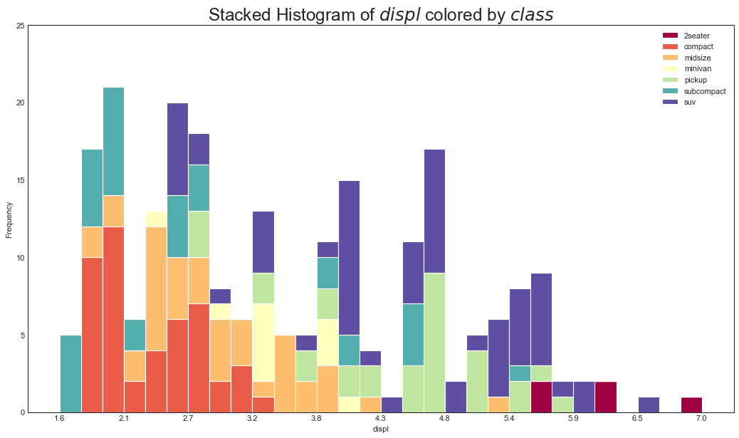
连续变量直方图(Histogram for Continuous Variable)
1
2
3
4
5
6
7
"""区别连续变量和分类变量"""
#数据准备
df = pd.read_csv("mpg_ggplot2.csv")
x_var = 'displ'
groupby_var = 'class'
df_agg = df.loc[:, [x_var, groupby_var]].groupby(groupby_var)
vals = [df[x_var].values.tolist() for i,df in df_agg]
1
2
3
4
5
6
7
8
9
10
11
12
13
14
15
16
17
18
19
20
#绘图
plt.figure(figsize=(16,9), dpi=80)
colors = [plt.cm.Spectral(i/float(len(vals)-1)) for i in range(len(vals))]
n, bins, patches = plt.hist(
    vals, 30, stacked=True, density=False, color=colors[:len(vals)]
)
#修饰图片
plt.legend(
    {group:col for group,col in \
    zip(np.unique(df[groupby_var]).tolist(), colors[:len(vals)])}
)
plt.title(
    f'Stacked Histogram of ${x_var}$ colored by ${groupby_var}$',
    fontsize=22
)
plt.xlabel(x_var)
plt.ylabel('Frequency')
plt.ylim(0, 25)
plt.xticks(ticks=bins[::3], labels=[round(b,1) for b in bins[::3]])
plt.show()
分类变量直方图(Histogram for Categorical Variable)
1
2
3
4
5
6
7
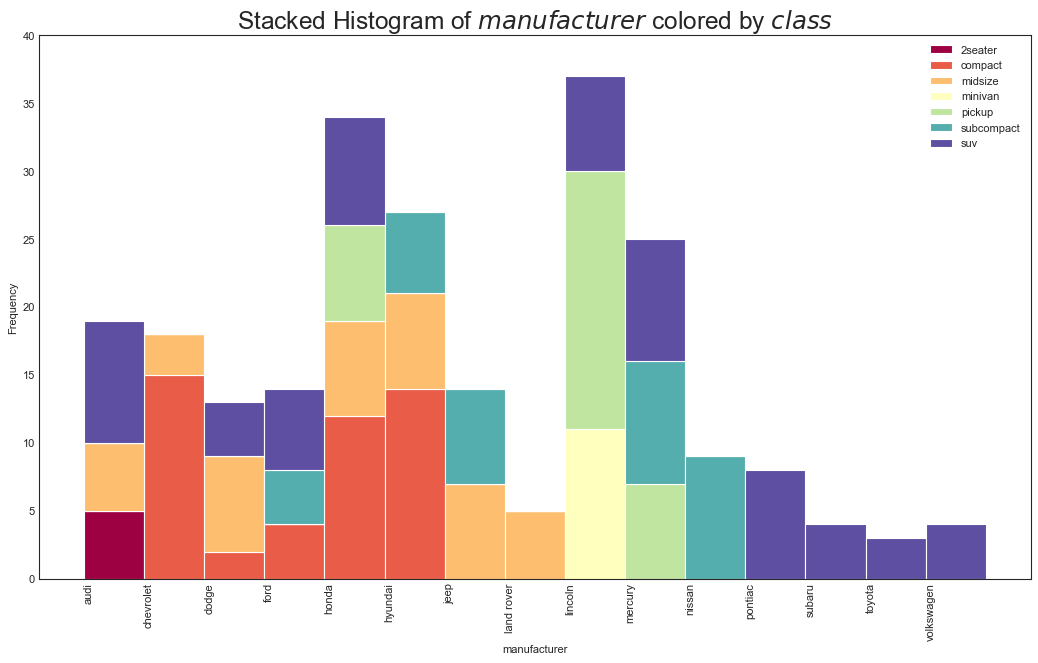
"""通过对条形图进行着色,可以将分布与表示颜色的另一个类型变量相关联"""
#数据准备
df = pd.read_csv("mpg_ggplot2.csv")
x_var = 'manufacturer'
groupby_var = 'class'
df_agg = df.loc[:, [x_var, groupby_var]].groupby(groupby_var)
vals = [df[x_var].values.tolist() for i,df in df_agg]
1
2
3
4
5
6
7
8
9
10
11
12
13
14
15
16
17
18
19
20
21
22
23
24
#绘图
plt.figure(figsize=(16,9), dpi=80)
colors = [plt.cm.Spectral(i/float(len(vals)-1)) for i in range(len(vals))]
n, bins, patches = plt.hist(
    vals, df[x_var].unique().__len__(),
    stacked=True, density=False, color=colors[:len(vals)]
)
#图片修饰
plt.legend(
    {group: col for group,col in \
    zip(np.unique(df[groupby_var]).tolist(), colors[:len(vals)])}
)
plt.title(
    f'Stacked Histogram of ${x_var}$ colored by ${groupby_var}$',
    fontsize=22
)
plt.xlabel(x_var)
plt.ylabel('Frequency')
plt.ylim(0, 40)
plt.xticks(
    ticks=bins, labels=np.unique(df[x_var]).tolist(),
    rotation=90, horizontalalignment='left'
)
plt.show()
密度图
1
2
3
4
5
6
7
8
9
10
11
12
13
14
15
16
17
18
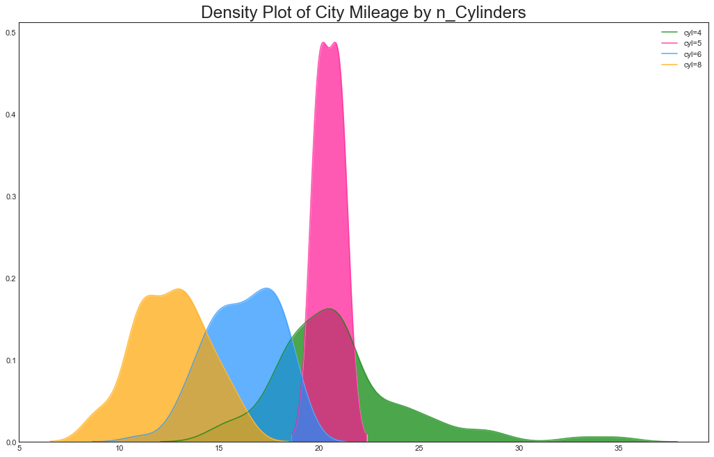
"""密度图用于可视化连续变量,通过‘响应’变量对它们进行分组。"""
#下例描述城市里程的分布如何随汽车缸数而变化
#数据准备
df = pd.read_csv('mpg_ggplot2.csv')
#绘图
plt.figure(figsize=(16,10), dpi=80)
sns.kdeplot(df.loc[df['cyl']==4, 'cty'], color='green', alpha=0.7,
label='cyl=4', shade=True)
sns.kdeplot(df.loc[df['cyl']==5, 'cty'], color='deeppink', alpha=0.7,
label='cyl=5', shade=True)
sns.kdeplot(df.loc[df['cyl']==6, 'cty'], color='dodgerblue', alpha=0.7,
label='cyl=6', shade=True)
sns.kdeplot(df.loc[df['cyl']==8, 'cty'], color='orange', alpha=0.7,
label='cyl=8', shade=True)
#修饰图片
plt.title("Density Plot of City Mileage by n_Cylinders", fontsize=22)
plt.legend()
plt.show()
直方密度线图(Density Curves with Histogran)
1
2
3
4
5
6
7
8
9
10
11
12
13
14
15
16
17
18
19
20
21
22
23
24
25
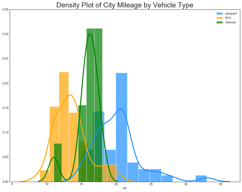
"""可以用一个图包含两个图所传达的集体信息"""
#数据准备
df = pd.read_csv('mpg_ggplot2.csv')
#绘图
plt.figure(figsize=(13,10), dpi=80)
sns.distplot(
df.loc[df['class']=='compact', 'cty'],
color='dodgerblue', label='compact',
hist_kws={'alpha': 0.7}, kde_kws={'linewidth': 3}
)
sns.distplot(
df.loc[df['class']=='suv', 'cty'],
color='orange', label='SUV',
hist_kws={'alpha': 0.7}, kde_kws={'linewidth': 3}
)
sns.distplot(
df.loc[df['class']=='minivan', 'cty'],
color='g', label="minivan",
hist_kws={'alpha': 0.7}, kde_kws={'linewidth': 3}
)
plt.ylim(0, 0.35)
#修饰
plt.title("Density Plot of City Mileage by Vehicle Type", fontsize=22)
plt.legend()
plt.show()
Joy Plot
1
2
3
4
5
6
7
8
9
10
11
12
13
14
15
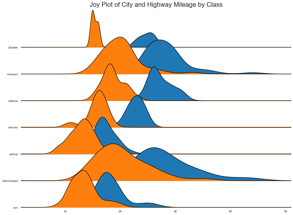
'''
Joy Plot 允许不同组的密度曲线重叠,这是一种可视化大量分组数据的彼此关系的好方法。
并且看起来更加悦目,更清晰地传达正确的信息
'''
import joypy
#数据准备
mpg = pd.read_csv("mpg_ggplot2.csv")
#绘图
plt.figure(figsize=(16,10), dpi=80)
fig, axes = joypy.joyplot(
mpg, column=['hwy', 'cty'], by='class', ylim='own', figsize=(14,10)
)
#修饰图片
plt.title("Joy Plot of City and Highway Mileage by Class", fontsize=22)
plt.show()
分布包点图(Distributed Dot Plot)
1
2
3
4
5
6
7
8
9
10
11
12
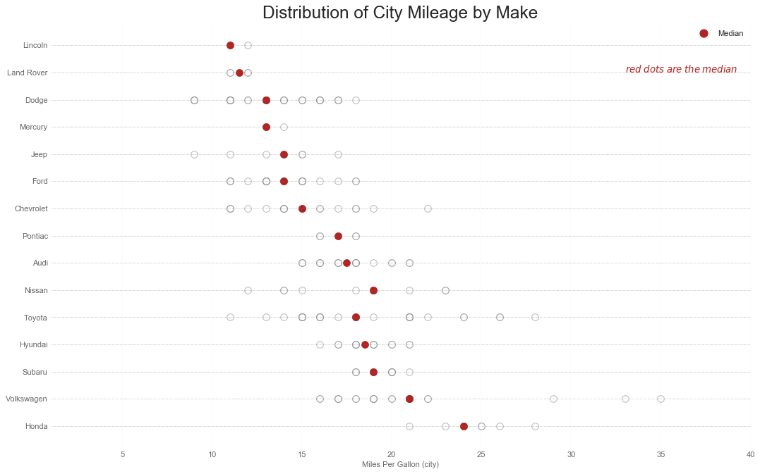
"""显示按组分割的点的单变量分布,点数越暗,集中度越高"""
from matplotlib import patches
#数据准备
df_raw = pd.read_csv("mpg_ggplot2.csv")
#在原始数据上添加一个与cyl匹配的color变量
cyl_colors = {4:'tab:red', 5:'tab:green', 6:'tab:blue', 8:'tab:orange'}
df_raw['cyl_color'] = df_raw.cyl.map(cyl_colors)
#计算均值和中位数
df = df_raw[['cty', 'manufacturer']].groupby('manufacturer').mean()
df.sort_values('cty', ascending=False, inplace=True)
df.reset_index(inplace=True)
df_median = df_raw[['cty', 'manufacturer']].groupby('manufacturer').median()
1
2
3
4
5
6
7
8
9
10
11
12
13
14
15
16
17
18
19
20
21
22
23
24
25
26
27
28
29
30
31
32
33
34
35
36
37
38
39
40
41
42
43
#绘图
fig, ax = plt.subplots(figsize=(16,10), dpi=80)
ax.hlines(
    y=df.index, xmin=0, xmax=40,
    color='gray', alpha=0.5, linewidth=0.5, linestyle='dashdot'
)
#画包点
for i,make in enumerate(df.manufacturer):
    df_make = df_raw.loc[df_raw.manufacturer==make, :]
    ax.scatter(
        y=np.repeat(i,df_make.shape[0]), x='cty', data=df_make,
        s=75, edgecolors='gray', c='w', alpha=0.5
    )
    ax.scatter(
        y=i, x='cty', data=df_median.loc[df_median.index==make, :],
        s=75, c='firebrick'
    )

#注释
ax.text(
    33, 13, "$red \; dots \; are \; the \: median$",
    fontsize=12, color='firebrick'
)

#修饰图片
red_patch = plt.plot([], [],
    marker='o', ms=10, ls='', mec=None, color='firebrick', label='Median')
plt.legend(handles=red_patch)
ax.set_title("Distribution of City Mileage by Make", fontsize=22)
ax.set_xlabel("Miles Per Gallon (city)", alpha=0.7)
ax.set_yticks(df.index)
ax.set_yticklabels(
    df.manufacturer.str.title(), alpha=0.7,
    fontdict={'horizontalalignment': 'right'}
)
ax.set_xlim(1, 40)
plt.xticks(alpha=0.7)
plt.gca().spines['top'].set_visible(False)
plt.gca().spines['bottom'].set_visible(False)
plt.gca().spines['right'].set_visible(False)
plt.gca().spines['left'].set_visible(False)
plt.grid(axis='both', alpha=0.4, linewidth=0.1)
plt.show()
箱形图
1
2
3
4
5
6
7
8
9
10
11
12
13
14
15
16
17
18
19
20
21
22
23
24
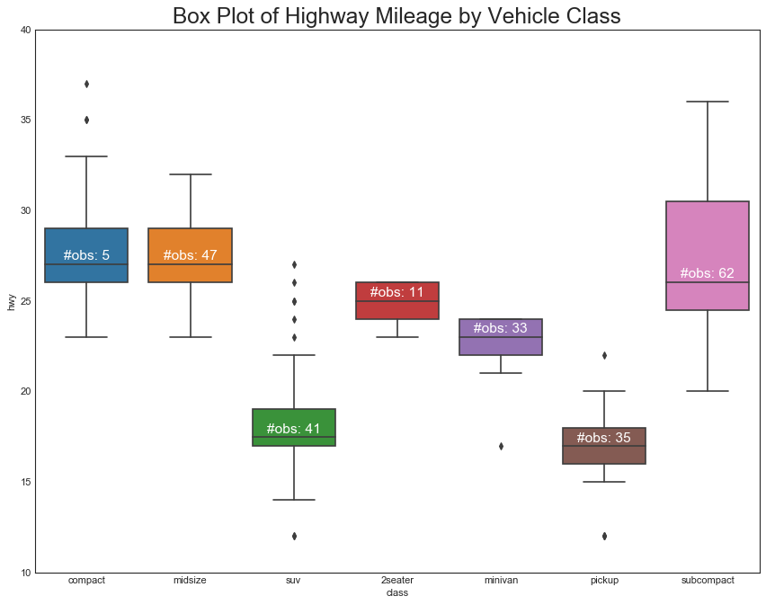
"""
绘制箱形图时需要注意解释可能会扭曲该组中包含的点数的框的大小
手动提供每个框中的观察数量,可以克服这个缺点
"""
#数据准备
df = pd.read_csv("mpg_ggplot2.csv")
#绘图
plt.figure(figsize=(13,10), dpi=80)
sns.boxplot(x='class', y='hwy', data=df, notch=False)
#在箱形图中添加N个obs(obtional)
def add_n_obs(df, group_var, y):
medians_dict = {grp[0]:grp[1][y].median() for grp in df.groupby(group_var)}
xticklabels = [x.get_text() for x in plt.gca().get_xticklabels()]
n_obs = df.groupby(group_var)[y].size().values
for (x, xticklabel),obs in zip(enumerate(xticklabels), n_obs):
plt.text(
x, medians_dict[xticklabel]*1.01, '#obs: '+str(obs),
horizontalalignment='center', fontsize=14, color='white'
)
add_n_obs(df, group_var='class', y='hwy')
#修饰图片
plt.title("Box Plot of Highway Mileage by Vehicle Class", fontsize=22)
plt.ylim(10, 40)
plt.show()
包点+箱形图(Dot+Box Plot)
1
2
3
4
5
6
7
8
9
10
11
12
13
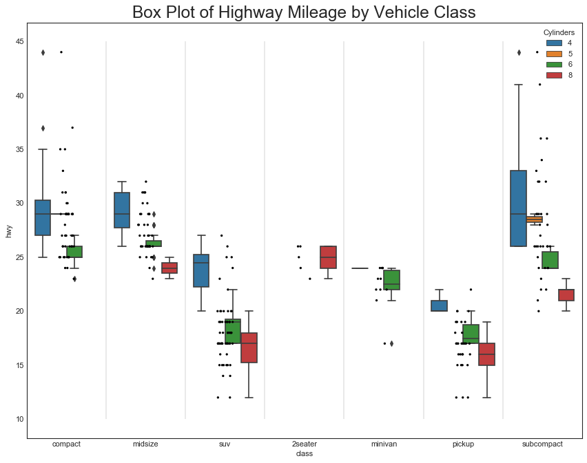
"""传达类似于分组的箱形图信息,此外还可以了解到每一组中的数据密度"""
#数据准备
df = pd.read_csv("mpg_ggplot2.csv")
#绘图
plt.figure(figsize=(13,10), dpi=80)
sns.boxplot(x='class', y='hwy', data=df, hue='cyl')
sns.stripplot(x='class', y='hwy', data=df, color='black', size=3, jitter=1)
for i in range(len(df["class"].unique())-1):
plt.vlines(i+0.5, 10, 45, linestyle='solid', colors='gray', alpha=0.2)
#修饰图片
plt.title("Box Plot of Highway Mileage by Vehicle Class", fontsize=22)
plt.legend(title='Cylinders')
plt.show()
小提琴图(Violin Plot)
1
2
3
4
5
6
7
df = pd.read_csv("mpg_ggplot2.csv")
#绘图
plt.figure(figsize=(13,10), dpi=80)
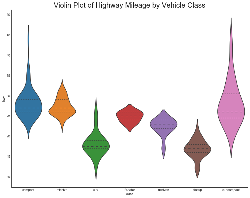
sns.violinplot(x='class', y='hwy', data=df, scale='width', inner='quartile')
#修饰图片
plt.title("Violin Plot of Highway Mileage by Vehicle Class", fontsize=22)
plt.show()
人口金字塔(Population Pyramid)
1
2
3
4
5
6
7
8
9
10
11
12
13
14
15
16
17
18
19
20
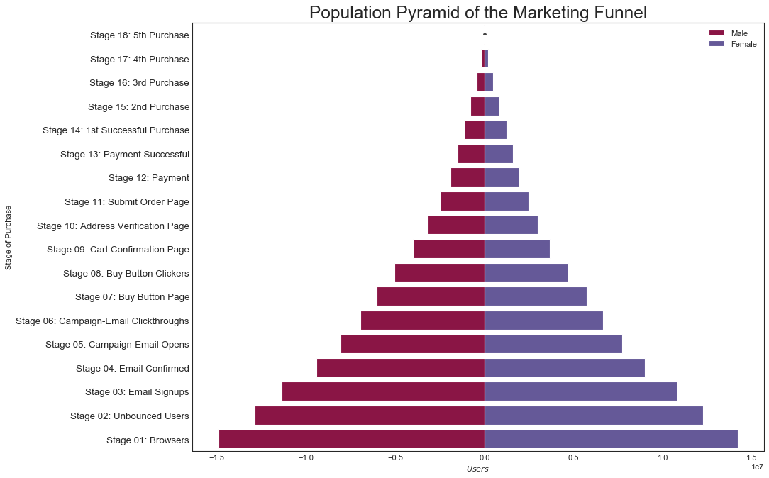
"""金字塔图可用于显示由数量排序的组的分布"""
df = pd.read_csv("email_campaign_funnel.csv")
#绘图
plt.figure(figsize=(13,10), dpi=80)
group_var = 'Gender'
order_of_bars = df.Stage.unique()[::-1]
colors = [plt.cm.Spectral(i/float(len(df[group_var].unique())-1)) for i in \
range(len(df[group_var].unique()))]
for c,group in zip(colors, df[group_var].unique()):
sns.barplot(
x='Users', y='Stage', data=df.loc[df[group_var]==group,:],
order=order_of_bars, color=c, label=group
)
#修饰图片
plt.xlabel("$Users$")
plt.ylabel('Stage of Purchase')
plt.yticks(fontsize=12)
plt.title("Population Pyramid of the Marketing Funnel", fontsize=22)
plt.legend()
plt.show()
分类图(Categorical Plots)
1
2
3
4
5
6
7
8
9
10
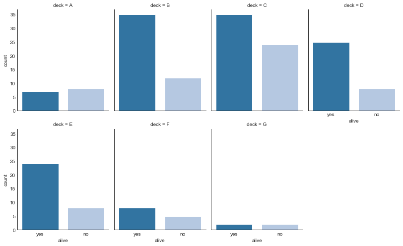
"""由seaborn库提供的,可用于可视化彼此相关的两个或多个分类变量的计数分布"""
#数据准备
titanic = sns.load_dataset('titanic')
#绘图
g = sns.catplot(
'alive', col='deck', col_wrap=4, kind='count', height=3.5,
aspect=0.8, palette='tab20', data=titanic[titanic.deck.notnull()]
)
fig.suptitle('sf')
plt.show()
1
2
3
4
5
6
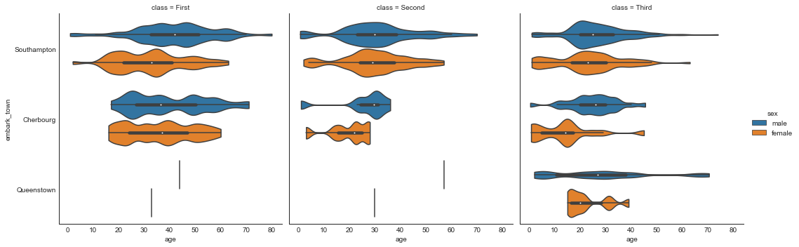
#绘图例2
sns.catplot(
x='age', y='embark_town', hue='sex', col='class', orient='h', height=5,
aspect=1, palette='tab10', kind='violin', dodge=True, cut=0, bw=0.2,
data=titanic[titanic.embark_town.notnull()]
)
五、组成(Composition)
华夫饼图(Waffle Chart)
1
2
3
4
5
6
7
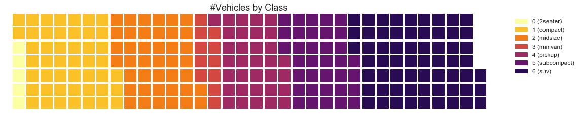
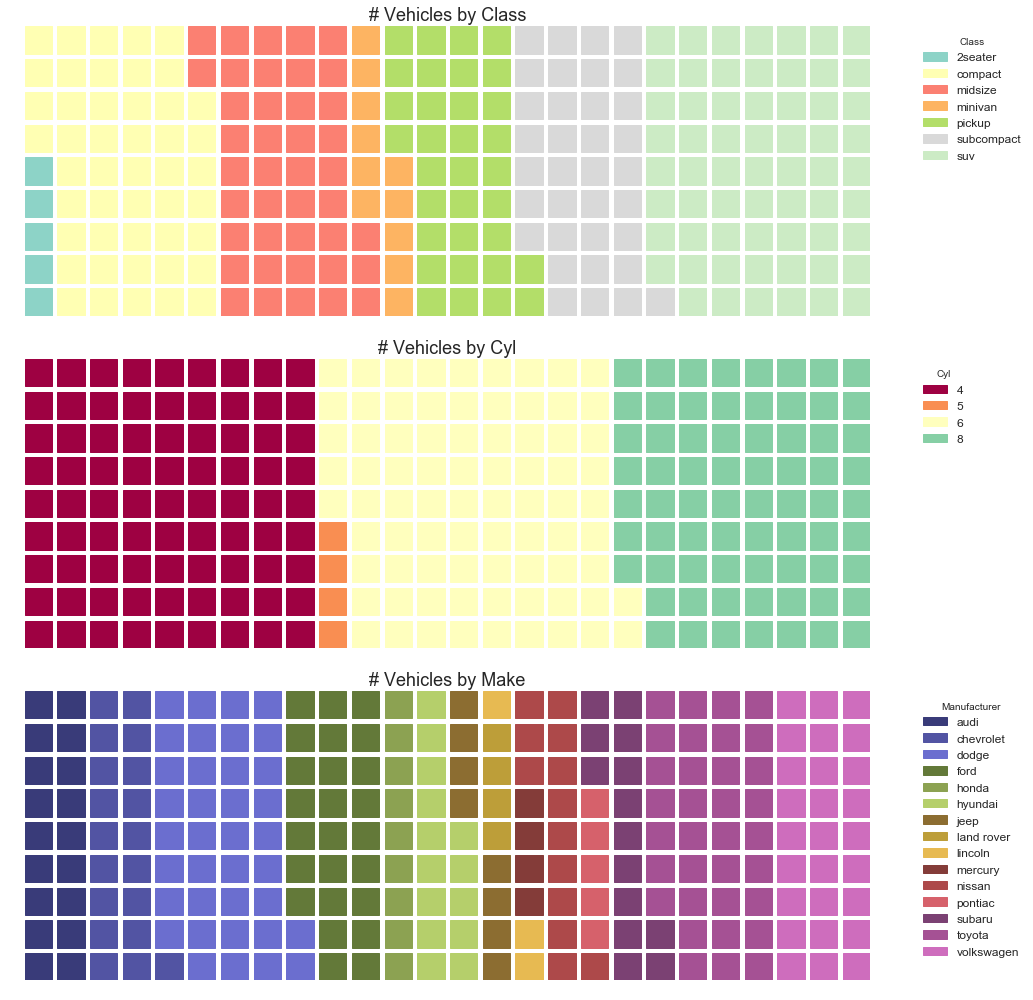
"""用于显示更大群体中的组的组成"""
from pywaffle import Waffle
#数据准备
df_raw = pd.read_csv("mpg_ggplot2.csv")
df = df_raw.groupby("class").size().reset_index(name='counts')
n_categories = df.shape[0]
colors = [plt.cm.inferno_r(i/float(n_categories)) for i in range(n_categories)]
1
2
3
4
5
6
7
8
9
10
11
12
13
14
15
16
17
#绘图
fig = plt.figure(
    FigureClass=Waffle, rows=7, colors=colors, figsize=(16,9),
    plots={
        '111': {
            'values': df["counts"],
            'labels': ["{0} ({1})".format(n[0], n[1]) for n in \
                df[['class', 'counts']].itertuples()],
            'legend': {
                'loc':'upper left', 'bbox_to_anchor':(1.05, 1), 'fontsize':12
            },
            'title': {
                'label':'#Vehicles by Class', 'loc':'center', 'fontsize':18
            }
        }
    }
)
1
2
3
4
5
6
7
8
9
10
11
12
13
14
#绘图例2----------------------------
#数据准备-------------
#By Class Data
df_class = df_raw.groupby("class").size().reset_index(name='counts_class')
cat_num = df_class.shape[0]
colors_class = [plt.cm.Set3(i/float(cat_num)) for i in range(cat_num)]
#By Cylinders Data
df_cyl = df_raw.groupby('cyl').size().reset_index(name='counts_cyl')
cat_num = df_cyl.shape[0]
colors_cyl = [plt.cm.Spectral(i/float(cat_num)) for i in range(cat_num)]
#By Make Data
df_make = df_raw.groupby('manufacturer').size().reset_index(name='counts_make')
cat_num = df_make.shape[0]
colors_make = [plt.cm.tab20b(i/float(cat_num)) for i in range(cat_num)]
1
2
3
4
5
6
7
8
9
10
11
12
13
14
15
16
17
18
19
20
21
22
23
24
25
26
27
28
29
30
31
32
33
34
35
36
37
38
39
40
41
42
43
44
45
46
47
#绘图
fig = plt.figure(
    FigureClass=Waffle,
    plots={
        '311': {
            'values': df_class['counts_class'],
            'labels': ["{1}".format(n[0], n[1]) for n in
                       df_class[['class', 'counts_class']].itertuples()],
            'legend': {
                'loc': 'upper left', 'bbox_to_anchor': (1.05, 1),
                'fontsize': 12, 'title':'Class'
            },
            'title': {
                'label':'# Vehicles by Class', 'loc':'center', 'fontsize':18
            },
            'colors': colors_class
        },
        '312': {
            'values': df_cyl['counts_cyl'],
            'labels': ["{1}".format(n[0], n[1]) for n in
                       df_cyl[['cyl', 'counts_cyl']].itertuples()],
            'legend': {
                'loc': 'upper left', 'bbox_to_anchor': (1.05, 1),
                'fontsize': 12, 'title':'Cyl'
            },
            'title': {
                'label':'# Vehicles by Cyl', 'loc':'center', 'fontsize':18
            },
            'colors': colors_cyl
        },
        '313': {
            'values': df_make['counts_make'],
            'labels': ["{1}".format(n[0], n[1]) for n in
                       df_make[['manufacturer', 'counts_make']].itertuples()],
            'legend': {
                'loc': 'upper left', 'bbox_to_anchor': (1.05, 1),
                'fontsize': 12, 'title':'Manufacturer'
            },
            'title': {
                'label':'# Vehicles by Make', 'loc':'center', 'fontsize':18
            },
            'colors': colors_make
        }
    },
    rows=9,
    figsize=(16, 14)
)
饼图(Pie Chart)
1
2
3
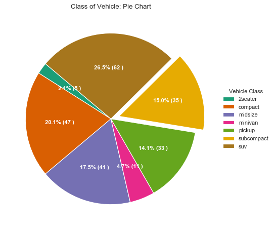
"""使用饼图最好标明百分比,否则饼图的面积可能存在误导"""
#数据准备
df_raw = pd.read_csv("mpg_ggplot2.csv")
1
2
3
4
5
6
df = df_raw.groupby("class").size()
#绘图例1
df.plot(kind='pie', subplots=True, figsize=(8, 8))
plt.title("Pie Chart of Vihecle Class - Bad")
plt.ylabel("")
plt.show()

1
2
3
4
5
6
7
8
df = df_raw.groupby('class').size().reset_index(name='counts')
data = df["counts"]
categories = df['class']
explode = [0,0,0,0,0,0.1,0]

def func(pct, allvals):
    absolute = int(pct/100.*np.sum(allvals))
    return "{:.1f}% ({:d} )".format(pct, absolute)
1
2
3
4
5
6
7
8
9
10
11
12
13
14
15
16
17
#绘图例2
fig, ax = plt.subplots(figsize=(12,7), subplot_kw=dict(aspect='equal'), dpi=80)

wedges, texts, autotexts = ax.pie(
    data, autopct=lambda pct: func(pct, data),
    textprops=dict(color='w'), colors=plt.cm.Dark2.colors,
    startangle=140, explode=explode
)

#修饰图片
ax.legend(
    wedges, categories, title='Vehicle Class',
    loc='center left', bbox_to_anchor=(1, 0, 0.5, 1)
)
plt.setp(autotexts, size=10, weight=700)
ax.set_title('Class of Vehicle: Pie Chart')
plt.show()
树形图(Treemap)
1
2
3
4
5
6
7
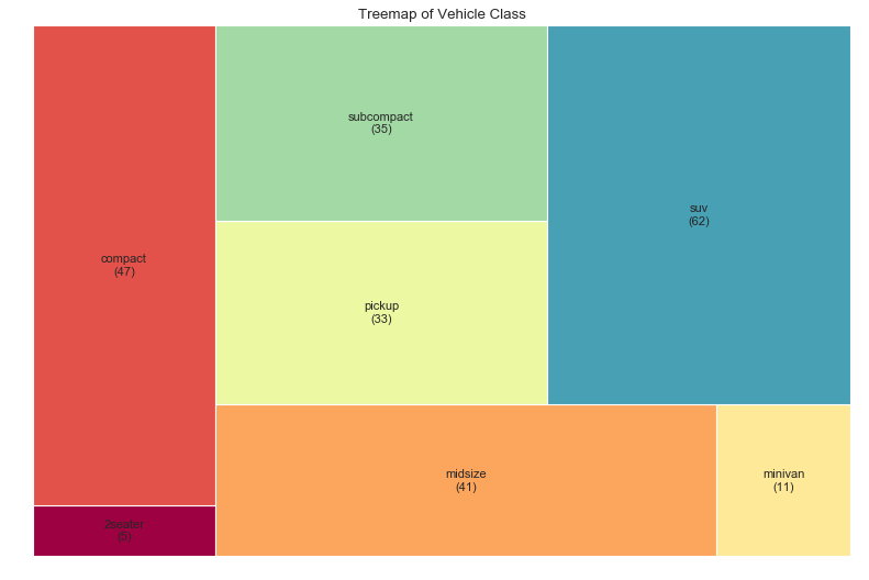
import squarify
#导入数据
df_raw = pd.read_csv('mpg_ggplot2.csv')
df = df_raw.groupby('class').size().reset_index(name='counts')
labels = df.apply(lambda x: str(x[0]) + '\n(' + str(x[1]) + ')', axis=1)
sizes = df['counts'].values.tolist()
colors = [plt.cm.Spectral(i/float(len(labels))) for i in range(len(labels))]
1
2
3
4
5
6
7
#绘图
plt.figure(figsize=(12,8), dpi=80)
squarify.plot(sizes=sizes, label=labels, color=colors)
#图片修饰
plt.title('Treemap of Vehicle Class')
plt.axis("off")
plt.show()
条形图(Bar Chart)
1
2
3
4
5
6
7
8
9
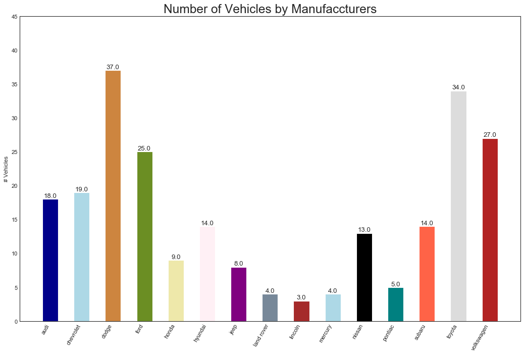
"""下面图表中,对每个项目使用了不同的颜色,颜色名称储存在all_colors变量中"""
import random
#数据导入
df_raw = pd.read_csv('mpg_ggplot2.csv')
df = df_raw.groupby("manufacturer").size().reset_index(name="counts")
n = df['manufacturer'].unique().__len__() + 1
all_colors = list(plt.cm.colors.cnames.keys())
random.seed(100)
c = random.choices(all_colors, k=n)
1
2
3
4
5
6
7
8
9
10
11
12
13
14
15
16
17
#绘图
plt.figure(figsize=(16, 10), dpi=80)
plt.bar(df["manufacturer"], df["counts"], color=c, width=0.5)
for i,val in enumerate(df["counts"].values):
    plt.text(
        i, val, float(val),
        horizontalalignment='center', verticalalignment='bottom',
        fontdict={"fontweight":500, "size":12}
    )
#修饰图片
plt.gca().set_xticklabels(
    df["manufacturer"], rotation=60, horizontalalignment='right'
)
plt.title("Number of Vehicles by Manufaccturers", fontsize=22)
plt.ylabel('# Vehicles')
plt.ylim(0, 45)
plt.show()
六、变化(Change)
时间序列图(Time Series Plot)
1
2
3
4
5
6
7
8
9
10
11
12
13
14
15
16
17
18
19
20
21
22
23
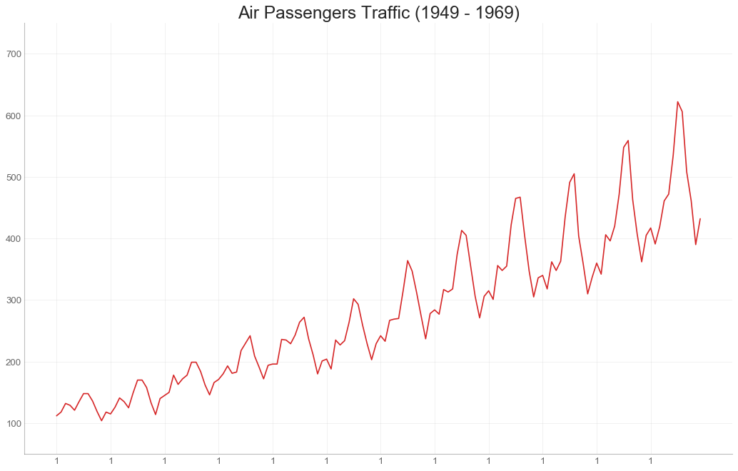
'''1949-1969年航空客运量的变化'''
#导入数据
df = pd.read_csv('AirPassengers.csv')
#绘图
plt.figure(figsize=(16, 10), dpi=80)
plt.plot('date', 'traffic', data=df, color='tab:red')
#修试图片
plt.ylim(50, 750)
xtick_location = df.index.tolist()[::12]
xtick_labels = [x[-4] for x in df.date.tolist()[::12]]
plt.xticks(
ticks=xtick_location, labels=xtick_labels,
rotation=0, fontsize=12, horizontalalignment='center', alpha=0.7
)
plt.yticks(fontsize=12, alpha=0.7)
plt.title("Air Passengers Traffic (1949 - 1969)", fontsize=22)
plt.grid(axis='both', alpha=0.3)
#remove borders
plt.gca().spines['top'].set_alpha(0)
plt.gca().spines['bottom'].set_alpha(0.3)
plt.gca().spines['right'].set_alpha(0)
plt.gca().spines['left'].set_alpha(0.3)
plt.show()
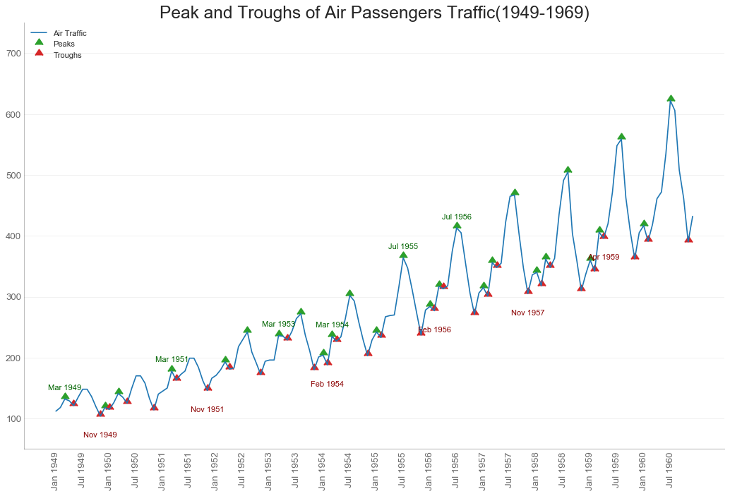
带波峰波谷标记的时序图(TS with Peaks and Troughs Annotated)
1
2
3
4
5
6
7
8
#导入数据
df = pd.read_csv('AirPassengers.csv')
#标记波峰和波谷
data = df['traffic'].values
doublediff = np.diff(np.sign(np.diff(data)))
peak_locations = np.where(doublediff == -2)[0] + 1
doublediff2 = np.diff(np.sign(np.diff(-1*data)))
trough_locations = np.where(doublediff2 == -2)[0] + 1
1
2
3
4
5
6
7
8
9
10
11
12
13
14
15
16
17
18
19
20
21
22
23
24
25
26
27
28
29
30
31
32
33
34
35
36
37
38
39
40
#绘图
plt.figure(figsize=(16, 10), dpi=80)
plt.plot('date', 'traffic', data=df, color='tab:blue', label='Air Traffic')
plt.scatter(
    df.date[peak_locations], df.traffic[peak_locations],
    marker= mpl.markers.CARETUPBASE, color='tab:green', s=100, label='Peaks'
)
plt.scatter(
    df.date[trough_locations], df.traffic[trough_locations],
    marker=mpl.markers.CARETUPBASE, color='tab:red', s=100, label='Troughs'
)
#注释
for t,p in zip(trough_locations[1::5], peak_locations[::3]):
    plt.text(
        df.date[p], df.traffic[p]+15, df.date[p],
        horizontalalignment='center', color='darkgreen'
    )
    plt.text(
        df.date[t], df.traffic[t]-35, df.date[t],
        horizontalalignment='center', color='darkred'
    )
#修饰图片
plt.ylim(50, 750)
xtick_location = df.index.tolist()[::6]
xtick_labels = df.date.tolist()[::6]
plt.xticks(
    ticks=xtick_location, labels=xtick_labels,
    rotation=90, fontsize=12, alpha=0.7
)
plt.title("Peak and Troughs of Air Passengers Traffic(1949-1969)", fontsize=22)
plt.yticks(fontsize=12, alpha=0.7)
#高亮边界
plt.gca().spines["top"].set_alpha(0)
plt.gca().spines["bottom"].set_alpha(0.3)
plt.gca().spines["right"].set_alpha(0)
plt.gca().spines["left"].set_alpha(0.3)

plt.legend(loc='upper left')
plt.grid(axis='y', alpha=0.3)
plt.show()
自相关和部分相关图( Autocorrelation(ACF) and Partial Autocorrelation(PACF) Plot)
1
2
3
4
5
6
7
8
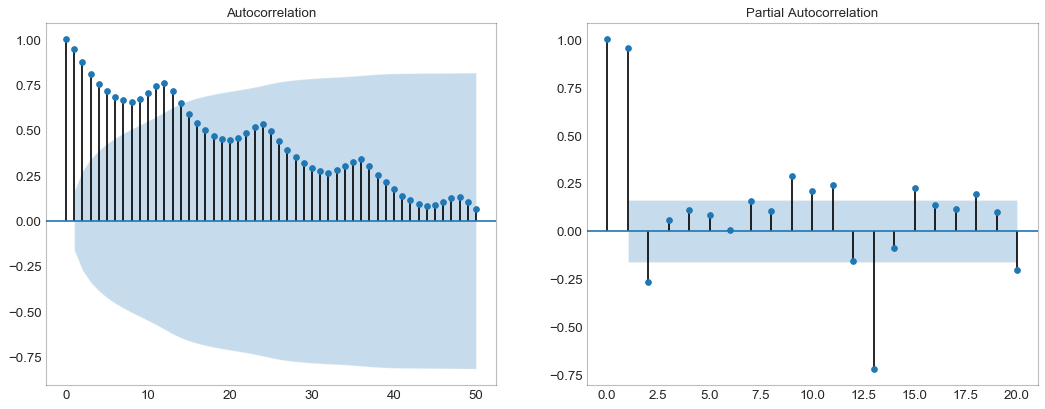
"""
自相关图(ACF)显示时间序列与其自身滞后的相关性,
图中蓝色阴影区域是显著性水平位于蓝线之上的滞后是显著的滞后。
PACF在另一方面显示了任何给定滞后与当前序列的自相关,但是删除了滞后的贡献。
"""
from statsmodels.graphics.tsaplots import plot_acf, plot_pacf
#数据导入
df = pd.read_csv("AirPassengers.csv")
1
2
3
4
5
6
7
8
9
10
11
12
13
#绘图
fig, (ax1, ax2) = plt.subplots(1, 2, figsize=(16, 6), dpi=80)
plot_acf(df.traffic.tolist(), ax=ax1, lags=50)
plot_pacf(df.traffic.tolist(), ax=ax2, lags=20)
#修饰图片
ax1.spines['top'].set_alpha(0.3); ax2.spines['top'].set_alpha(0.3)
ax1.spines['bottom'].set_alpha(0.3); ax2.spines['bottom'].set_alpha(0.3)
ax1.spines['right'].set_alpha(0.3); ax2.spines['right'].set_alpha(0.3)
ax1.spines['left'].set_alpha(0.3); ax2.spines['left'].set_alpha(0.3)

ax1.tick_params(axis='both', labelsize=12)
ax2.tick_params(axis='both', labelsize=12)
plt.show()
交叉相关图(Cross Correlation Plot)
1
2
3
4
5
6
7
8
9
10
11
12
13
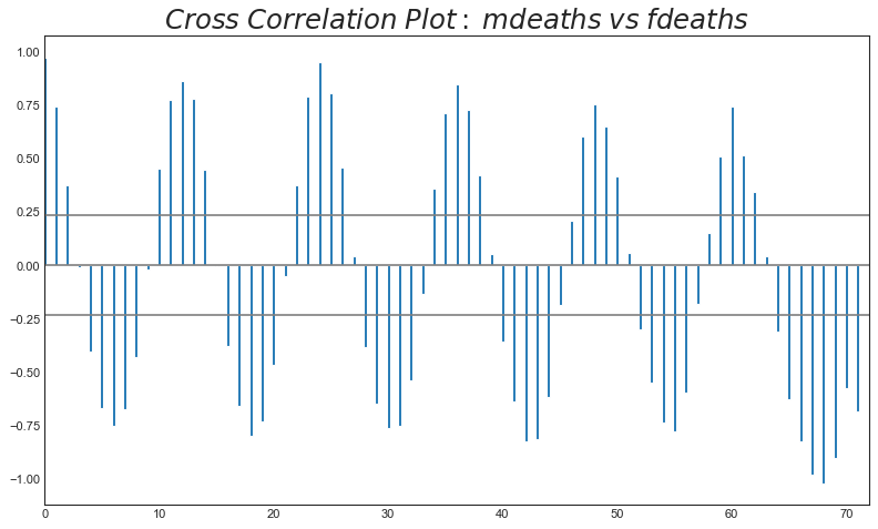
'''交叉相关图显示了两个时间序列相互之间的之后'''
import statsmodels.tsa.stattools as stattools
#数据准备
df = pd.read_csv("mortality.csv")
x = df["mdeaths"]
y = df["fdeaths"]
#计算交叉相关(Cross Correlation)
ccs = stattools.ccf(x, y)[:100]
nlags = len(ccs)
#计算显著性水平(significance level)
# https://stats.stackexchange.com/questions/3115/
# cross-correlation-significance-in-r/3128#3128
conf_level = 2/np.sqrt(nlags)
1
2
3
4
5
6
7
8
9
10
11
12
13
#绘图
plt.figure(figsize=(12,7), dpi=80)

plt.hlines(0, xmin=0, xmax=100, color='gray')
plt.hlines(conf_level, xmin=0, xmax=100, color='gray')
plt.hlines(-conf_level, xmin=0, xmax=100, color='gray')

plt.bar(x=np.arange(len(ccs)), height=ccs, width=0.3)

#修饰图片
plt.title('$Cross\; Correlation\; Plot:\; mdeaths\; vs\; fdeaths$', fontsize=22)
plt.xlim(0, len(ccs))
plt.show()
时间序列分解图(TS Decomposition Plot)
1
2
3
4
5
6
7
8
9
10
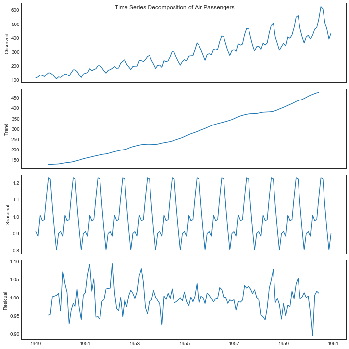
'''时间序列分解图显示时间序列的分解趋势,季节和残差分量'''
from statsmodels.tsa.seasonal import seasonal_decompose
from dateutil.parser import parse
#数据准备
df = pd.read_csv('AirPassengers.csv')
#修改日期格式
dates = pd.DatetimeIndex([parse(d).strftime('%Y-%m-01') for d in df['date']])
df.set_index(dates, inplace=True)
#分解
result = seasonal_decompose(df['traffic'], model='multiplicative')
1
2
3
4
#绘图
plt.rcParams.update({'figure.figsize': (10,10)})
result.plot().suptitle('Time Series Decomposition of Air Passengers')
plt.show()
多个时间序列(Multiple Time Series)
1
2
3
4
5
6
7
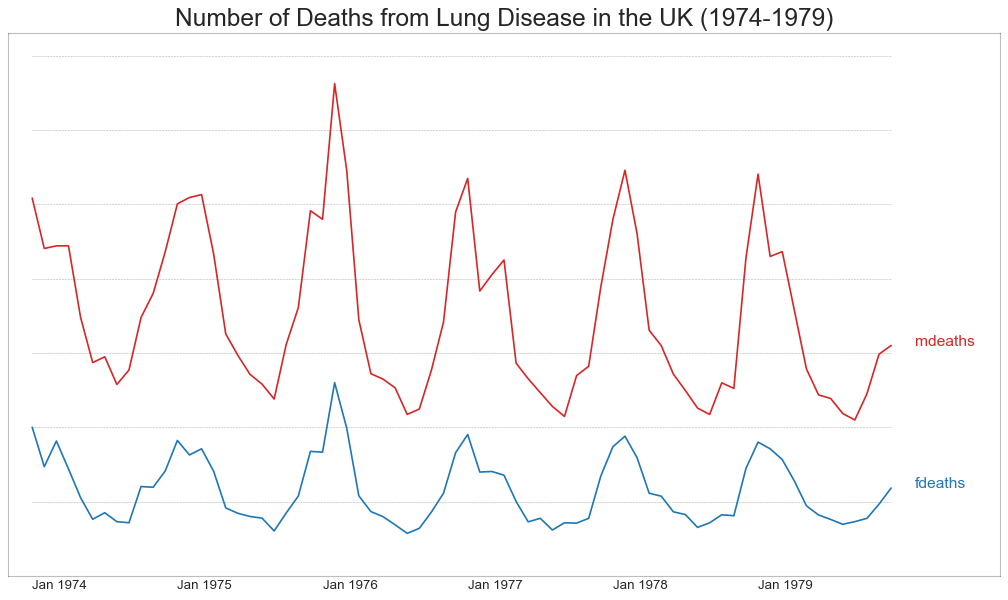
'''绘制多个序列,在同一个图表上测量相同的值'''
df = pd.read_csv('mortality.csv')
#定义 upper limit, lower limit, Y轴区间, 以及颜色
y_LL = 100
y_UL = int(df.iloc[:, 1:].max().max()*1.1)
y_interval = 400
mycolors = ['tab:red', 'tab:blue', 'tab:green', 'tab:orange']
1
2
3
4
5
6
7
8
9
10
11
12
13
14
15
16
17
18
19
20
21
22
23
24
25
26
27
28
29
30
31
32
33
34
35
36
37
38
39
40
#绘图与注释
fig, ax = plt.subplots(1, 1, figsize=(16,9), dpi=80)
columns = df.columns[1:]
for i,column in enumerate(columns):
    plt.plot(df.date.values, df[column].values, lw=1.5, color=mycolors[i])
    plt.text(
        df.shape[0] + 1, df[column].values[-1], column,
        fontsize=14, color=mycolors[i]
    )
#draw tick lines
for y in range(y_LL, y_UL, y_interval):
    plt.hlines(
        y, xmin=0, xmax=71,
        colors='black', alpha=0.3, linestyle='--', lw=0.5
    )
#高亮边界
plt.gca().spines['top'].set_alpha(0.3)
plt.gca().spines['bottom'].set_alpha(0.3)
plt.gca().spines['right'].set_alpha(0.3)
plt.gca().spines['left'].set_alpha(0.3)
#修饰图片
plt.tick_params(
    axis='both', which='both', bottom=False, top=False,
    labelbottom=True, left=False, right=False, labelleft=False
)
plt.title(
    'Number of Deaths from Lung Disease in the UK (1974-1979)',
    fontsize=22
)
plt.yticks(
    range(y_LL, y_UL, y_interval),
    [str(y) for y in range(y_LL, y_UL, y_interval)], fontsize=22
    )
plt.xticks(
    range(0, df.shape[0], 12),
    df.date.values[::12], horizontalalignment='left', fontsize=12
)
plt.ylim(y_LL, y_UL)
plt.xlim(-2, 80)
plt.show()
使用辅助Y轴来绘制不同范围的图形
1
2
3
4
5
6
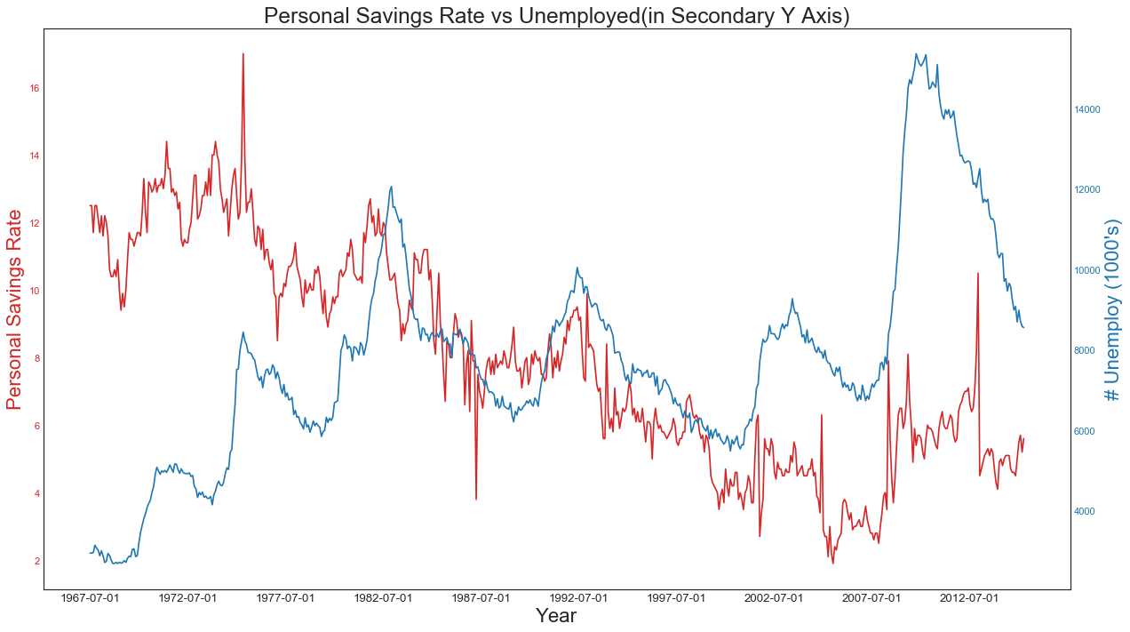
'''如果要显示在同一时间点度量两个不同数量的时间序列,可以绘制辅助Y轴'''
#数据准备
df = pd.read_csv("economics.csv")
x = df['date']
y1 = df['psavert']
y2 = df['unemploy']
1
2
3
4
5
6
7
8
9
10
11
12
13
14
15
16
17
18
19
20
21
22
#绘图1
fig, ax1 = plt.subplots(1, 1, figsize=(16,9), dpi=80)
ax1.plot(x, y1, color='tab:red')
#绘图2
ax2 = ax1.twinx()
ax2.plot(x, y2, color='tab:blue')
#ax1修饰
ax1.set_xlabel('Year', fontsize=20)
ax1.tick_params(axis='x', rotation=0, labelsize=12)
ax1.set_ylabel('Personal Savings Rate', color='tab:red', fontsize=20)
ax1.tick_params(axis='y', rotation=0, labelcolor='tab:red')
#ax2修饰
ax2.set_ylabel("# Unemploy (1000's)", color='tab:blue', fontsize=20)
ax2.tick_params(axis='y', labelcolor='tab:blue')
ax2.set_xticks(np.arange(0,len(x),60))
ax2.set_xticklabels(x[::60], rotation=90, fontsize=10)
ax2.set_title(
    'Personal Savings Rate vs Unemployed(in Secondary Y Axis)',
    fontsize=22
)
fig.tight_layout()
plt.show()
带有误差带的时间序列(TS with Error Bands)
1
2
3
4
5
6
7
8
9
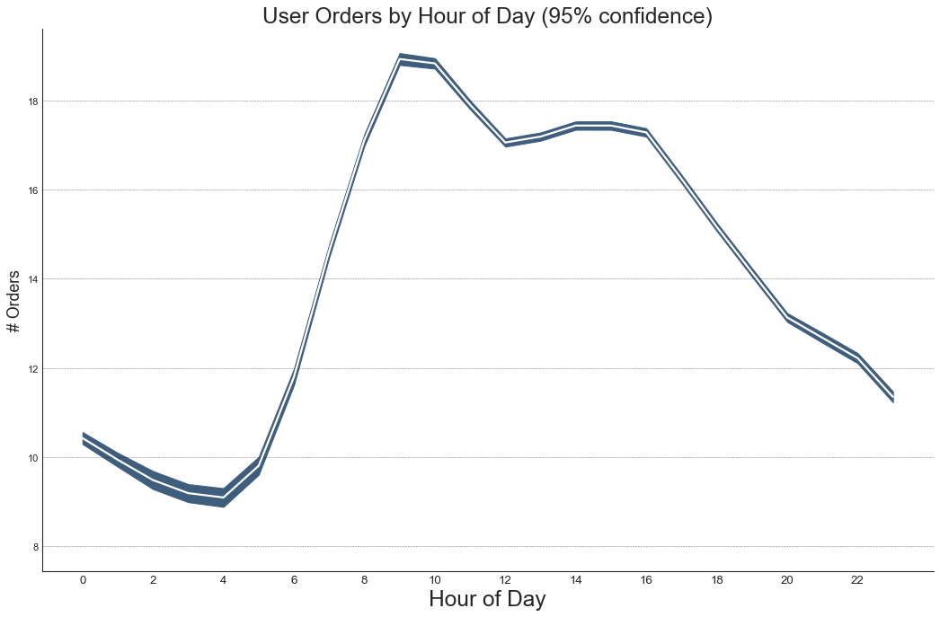
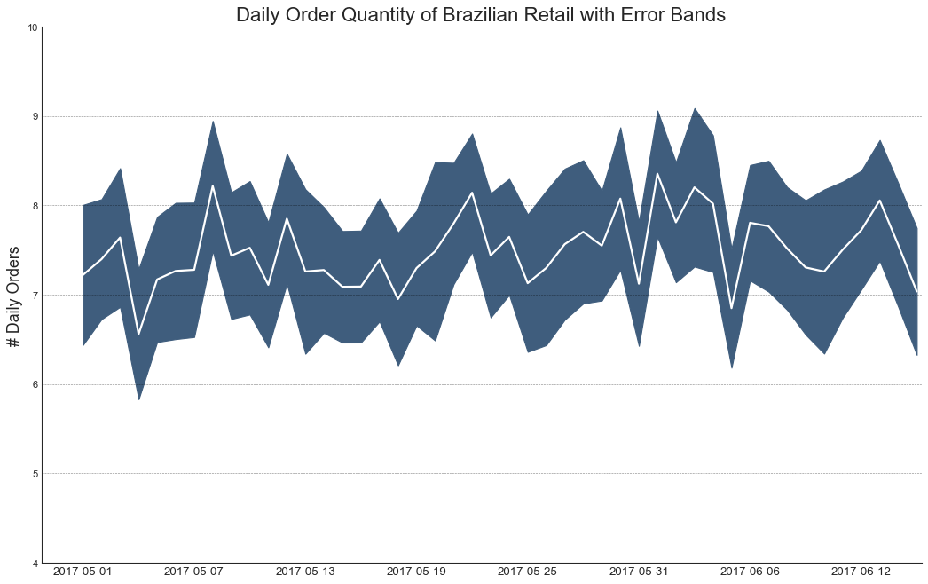
"""
如果有一个时间序列,每个时间点有多个观测值,可使用带有误差带的时间序列图。
在下图中订单数量的平均值由白线表示,并且围绕均值绘制95%的置信区间
"""
from scipy.stats import sem
#数据准备
df = pd.read_csv('user_orders_hourofday.csv')
df_mean = df.groupby('order_hour_of_day').quantity.mean()
df_se = df.groupby('order_hour_of_day').quantity.apply(sem).mul(1.96)
1
2
3
4
5
6
7
8
9
10
11
12
13
14
15
16
17
18
19
20
21
22
23
24
25
26
27
#绘图
plt.figure(figsize=(16,10), dpi=80)
plt.ylabel('# Orders', fontsize=16)
x = df_mean.index
plt.plot(x, df_mean, color='white', lw=2)
plt.fill_between(x, df_mean-df_se, df_mean+df_se, color='#3F5D7D')

#高亮边界
plt.gca().spines['top'].set_alpha(0)
plt.gca().spines['bottom'].set_alpha(1)
plt.gca().spines['right'].set_alpha(0)
plt.gca().spines['left'].set_alpha(1)

#修饰图片
plt.xticks(x[::2], [str(d) for d in x[::2]], fontsize=12)
plt.title('User Orders by Hour of Day (95% confidence)', fontsize=22)
plt.xlabel('Hour of Day', fontsize=22)

s, e = plt.gca().get_xlim()
plt.xlim(s, e)

#绘制水平标记线
for y in range(8, 20, 2):
    plt.hlines(
        y, xmin=s, xmax=e, color='black', alpha=0.5, linestyle='--', lw=0.5
    )
plt.show()
1
2
3
4
5
6
7
8
9
'''第二个例子'''
from dateutil.parser import parse
from scipy.stats import sem
#数据准备
df_raw = pd.read_csv(
    'orders_45d.csv', parse_dates=['purchase_time','purchase_date']
)
df_mean = df_raw.groupby('purchase_date').quantity.mean()
df_se = df_raw.groupby('purchase_date').quantity.apply(sem).mul(1.96)
1
2
3
4
5
6
7
8
9
10
11
12
13
14
15
16
17
18
19
20
21
22
23
24
25
26
27
28
29
#绘图
plt.figure(figsize=(16,10), dpi=80)
plt.ylabel('# Daily Orders', fontsize=16)
x = [d.date().strftime('%Y-%m-%d') for d in df_mean.index]
plt.plot(x, df_mean, color='white', lw=2)
plt.fill_between(x, df_mean-df_se, df_mean+df_se, color='#3F5D7D')

#高亮边界
plt.gca().spines['top'].set_alpha(0)
plt.gca().spines['bottom'].set_alpha(1)
plt.gca().spines['right'].set_alpha(0)
plt.gca().spines['left'].set_alpha(1)

#修饰图片
plt.xticks(x[::6], [str(d) for d in x[::6]], fontsize=12)
plt.title(
    'Daily Order Quantity of Brazilian Retail with Error Bands',
    fontsize=20
)
s, e = plt.gca().get_xlim()
plt.xlim(s, e-2)
plt.ylim(4, 10)

for y in range(5, 10, 1):
    plt.hlines(
        y, xmin=s ,xmax=e,
        colors='black', alpha=0.5, linestyle='--', lw=0.5
    )
plt.show()
堆积面积图(Stacked Area Chart)
1
2
3
4
5
6
7
8
9
10
11
12
13
14
15
16
17
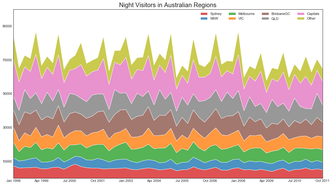
'''可以直观地显示多个时间序列的贡献程度,更容易进行比较'''
#数据准备
df = pd.read_csv('nightvisitors.csv')
mycolors = [
'tab:red', 'tab:blue', 'tab:green', 'tab:orange',
'tab:brown', 'tab:grey', 'tab:pink', 'tab:olive'
]
x = df['yearmon'].values.tolist()
y0 = df[columns[0]].values.tolist()
y1 = df[columns[1]].values.tolist()
y2 = df[columns[2]].values.tolist()
y3 = df[columns[3]].values.tolist()
y4 = df[columns[4]].values.tolist()
y5 = df[columns[5]].values.tolist()
y6 = df[columns[6]].values.tolist()
y7 = df[columns[7]].values.tolist()
y = np.vstack([y0, y2, y4, y6, y7, y5, y1, y3])
1
2
3
4
5
6
7
8
9
10
11
12
13
14
15
16
17
#绘图
fig, ax = plt.subplots(1, 1, figsize=(16,9), dpi=80)

#对每一列进行绘图
columns = df.columns[1:]
labs = columns.values.tolist()
ax = plt.gca()
ax.stackplot(x, y, labels=labs, colors=mycolors, alpha=0.8)

#修饰图片
ax.set_title('Night Visitors in Australian Regions', fontsize=18)
ax.set(ylim=[0,100000])
ax.legend(fontsize=10, ncol=4)
plt.xticks(x[::5], fontsize=10, horizontalalignment='center')
plt.yticks(np.arange(10000,100000,20000), fontsize=10)
plt.xlim(x[0], x[-1])
plt.show()
未堆积的面积图(Unstacked Area Chart)
1
2
3
4
5
6
7
8
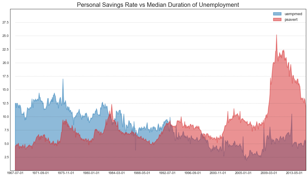
"""适用于可视化两个或多个系列相对于彼此的起伏情况"""
# 下图展示了随着失业率的增加,个人储蓄率的下降
#数据准备
df = pd.read_csv('economics.csv')
x = df['date'].values.tolist()
y1 = df['psavert'].values.tolist()
y2 = df['uempmed'].values.tolist()
columns = ['psavert', 'uempmed']
1
2
3
4
5
6
7
8
9
10
11
12
13
14
15
16
17
18
19
20
21
22
23
24
25
#绘图
fig, ax = plt.subplots(1, 1, figsize=(16,9), dpi=80)
ax.fill_between(
    x, y1=y1, y2=0,
    label=columns[1], alpha=0.5, color=mycolors[1], linewidth=2
)
ax.fill_between(
    x, y1=y2, y2=0,
    label=columns[0], alpha=0.5, color=mycolors[0], linewidth=2
)
#修饰图片
ax.set_title(
    "Personal Savings Rate vs Median Duration of Unemployment", fontsize=18
)
ax.set(ylim=[0,30])
ax.legend(loc='best', fontsize=12)
plt.xticks(x[::50], fontsize=10, horizontalalignment='center')
plt.yticks(np.arange(2.5,30.0,2.5), fontsize=10)
plt.xlim(-10, x[-1])
for y in np.arange(2.5, 30.0, 2.5):
    plt.hlines(
        y, xmin=0, xmax=len(x),
        colors='black', alpha=0.3, linestyles='--', lw=0.5
    )
plt.show()
日历热力图(Calendar Heat Map)
1
2
3
4
5
6
7
8
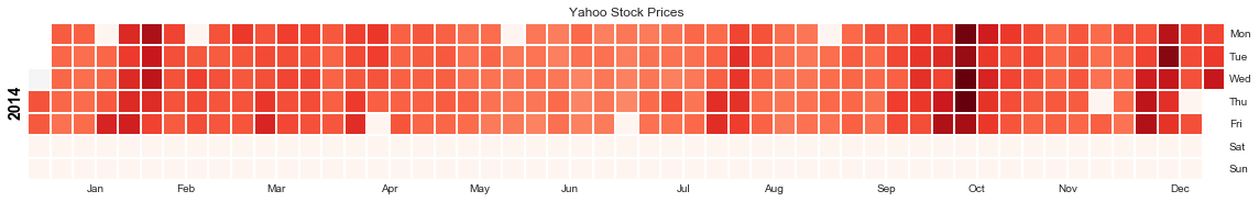
"""
日历热力图是可视化基于时间的数据次优选择,虽然视觉上好看,但是数值并不十分明显,
优点是可以很好地描绘极端值和假日效应
"""
import calmap
#数据准备
df = pd.read_csv('yahoo.csv', parse_dates=['date'])
df.set_index('date', inplace=True)
1
2
3
4
5
6
7
8
9
#绘图
plt.figure(figsize=(16,10), dpi=80)
calmap.calendarplot(
    df['2014']['VIX.Close'],
    fig_kws={'figsize': (16,10)},
    yearlabel_kws={'color': 'black', 'fontsize': 14},
    subplot_kws={'title': 'Yahoo Stock Prices'}
)
plt.show()
季节图(Seasonal Plot)
1
2
3
4
5
6
7
8
9
10
11
12
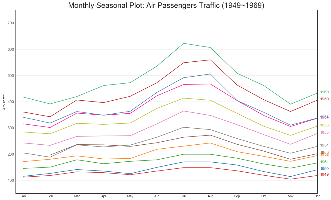
"""季节图可用于比较上一季中同一天的时间序列"""
from dateutil.parser import parse
#数据准备
df = pd.read_csv('AirPassengers.csv')
df['year'] = [parse(d).year for d in df.date]
df['month'] = [parse(d).strftime('%b') for d in df.date]
years = df['year'].unique()
mycolors = [
'tab:red', 'tab:blue', 'tab:green', 'tab:orange', 'tab:brown',
'tab:grey', 'tab:pink', 'tab:olive', 'deeppink', 'steelblue',
'firebrick', 'mediumseagreen'
]
1
2
3
4
5
6
7
8
9
10
11
12
13
14
15
16
17
18
19
20
21
22
23
24
#绘图
plt.figure(figsize=(16,10), dpi=80)
for i,y in enumerate(years):
    plt.plot(
        'month', 'traffic', data=df.loc[df.year==y, :],
        color=mycolors[i], label=y
    )
    plt.text(
        df.loc[df.year==y, :].shape[0]-0.9,
        df.loc[df.year==y, 'traffic'][-1:].values[0],
        y, fontsize=12, color=mycolors[i]
    )

#修饰图片
plt.ylim(50, 750)
plt.xlim(-0.3, 11)
plt.ylabel('$Air Traffic$')
plt.yticks(fontsize=12, alpha=0.7)
plt.title(
    "Monthly Seasonal Plot: Air Passengers Traffic (1949~1969)",
    fontsize=22
)
plt.grid(axis='y', alpha=0.3)
plt.show()
七、分组(Groups)
树状图(Dendrogram)
1
2
3
4
5
6
7
8
9
10
11
12
13
14
15
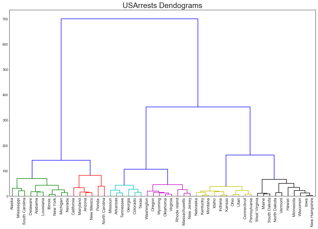
"""
树状图基于给定的距离度量将相似的点组合在一起,并基于点的相似性组织在树状链接中
"""
import scipy.cluster.hierarchy as sch
#数据准备
df = pd.read_csv("USArrests.csv")
#绘图
plt.figure(figsize=(16,10), dpi=80)
plt.title('USArrests Dendograms', fontsize=22)
dend = sch.dendrogram(
sch.linkage(df[['Murder','Assault','UrbanPop','Rape']], method='ward'),
labels=df.State.values, color_threshold=100
)
plt.xticks(fontsize=12)
plt.show()
簇状图(Cluster Plot)
1
2
3
4
5
6
7
8
9
10
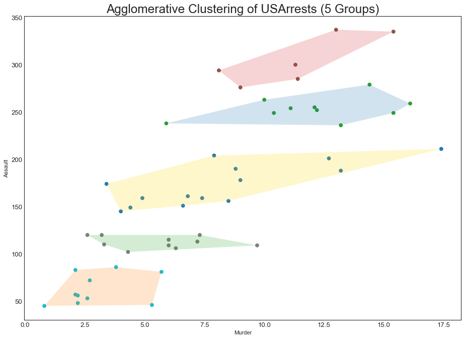
"""用于划分属于同一群集的点"""
from sklearn.cluster import AgglomerativeClustering
from scipy.spatial import ConvexHull
#数据准备
df = pd.read_csv("USArrests.csv")
#划分聚类
cluster = AgglomerativeClustering(
n_clusters=5, affinity='euclidean', linkage='ward'
)
cluster.fit_predict(df[['Murder', 'Assault', 'UrbanPop', 'Rape']])
1
2
3
4
5
6
7
#Encircle
def encircle(x, y, ax=None, **kw):
    if not ax: ax=plt.gca()
    p = np.c_[x, y]
    hull = ConvexHull(p)
    poly = plt.Polygon(p[hull.vertices,:], **kw)
    ax.add_patch(poly)
1
2
3
4
5
6
7
8
9
10
11
12
13
14
15
16
17
18
#绘图
plt.figure(figsize=(14,10), dpi=80)
plt.scatter(df.iloc[:,0], df.iloc[:,1], c=cluster.labels_, cmap='tab10')
#围绕顶点绘制多边形
colors = ['gold', 'tab:blue', 'tab:red', 'tab:green', 'tab:orange']
def plot_poly(label, fc):
    encircle(
        df.loc[cluster.labels_ == label, 'Murder'],
        df.loc[cluster.labels_ == label, 'Assault'],
        ec="k", fc=fc, alpha=0.2, linewidth=0
    )
for label, fc in zip(range(5), colors):
    plot_poly(label, fc)
#修饰图片
plt.xlabel('Murder'); plt.xticks(fontsize=12)
plt.ylabel('Assault'); plt.yticks(fontsize=12)
plt.title("Agglomerative Clustering of USArrests (5 Groups)", fontsize=22)
plt.show()
安德鲁斯曲线(Andrews Curve)
1
2
3
4
5
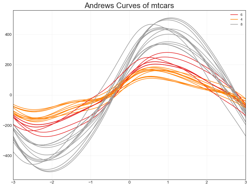
"""Andrew曲线有助于可视化是否存在基于给定分组的数字特征的固定分组"""
from pandas.plotting import andrews_curves
#数据准备
df = pd.read_csv("mtcars.csv")
df.drop(['cars', 'carname'], axis=1, inplace=True)
1
2
3
4
5
6
7
8
9
#绘图
plt.figure(figsize=(12,9), dpi=80)
andrews_curves(df, 'cyl', colormap='Set1')
#修饰
plt.title("Andrews Curves of mtcars", fontsize=22)
plt.xlim(-3, 3)
plt.grid(alpha=0.3)
plt.xticks(fontsize=12); plt.yticks(fontsize=12)
plt.show()
平行坐标(Parallel Coordinates)
1
2
3
4
5
6
7
8
9
10
11
12
13
14
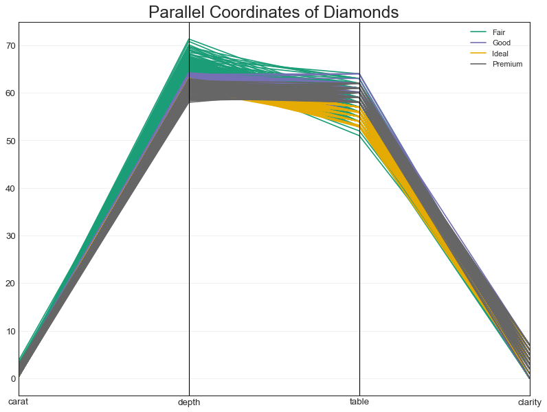
"""
判断特征是否有助于有效地隔离组,如果实现隔离,则该特征在预测该组时非常有用
"""
from pandas.plotting import parallel_coordinates
#数据准备
df_final = pd.read_csv("diamonds_filter.csv")
#绘图
plt.figure(figsize=(12,9), dpi=80)
parallel_coordinates(df_final, 'cut', colormap='Dark2')
#修饰
plt.title("Parallel Coordinates of Diamonds", fontsize=22)
plt.grid(alpha=0.3)
plt.xticks(fontsize=12); plt.yticks(fontsize=12)
plt.show()