简介
这本书比较冷门,因为需要快速上手 python 机器学习,随便找本书来学习一下。虽然内容比较浅显,不够深入,但是作为快速上手的教材很好用。其实整本书就是相当于 scikit-learn 的一个帮助文档而已,没有扯什么原理性的东西。如果有一定基础,要熟悉 scikit-learn,其实就是拿速查表刷一遍就行了:
本书前三章介绍 Python 编程的基础和数据处理、数据分析的基础,比较熟悉的内容,直接跳过。记录一下后面几章的学习笔记。文中涉及的算法原理可以参考另一个系列笔记:
R 统计学习(ISLR)– Learning Notes(I)
第四章 数据分析 – 深入理解
(1)主成分分析
- 对于多变量问题,进行 PCA 降维只有很小的信息损失。
- 对于一维数据,使用方差衡量数据的变异情况;对于多维数据,使用协方差矩阵。
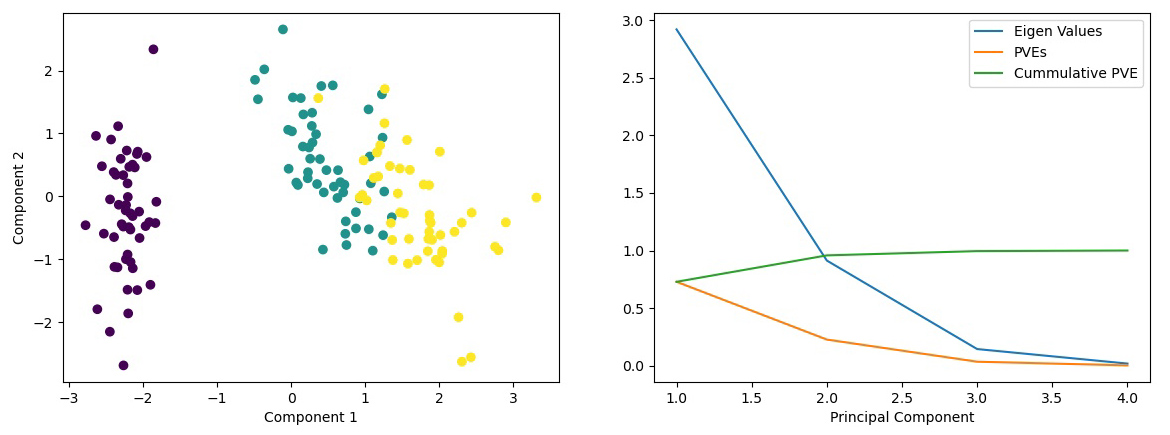
- 示例:在 iris 数据集上进行 PCA 降维:
- 数据标准化:均值为 0,方差为 1
- 计算数据的相关矩阵和单位标准差偏差值
- 将相关矩阵分解成特征向量和特征值
- 根据特征值的大小,选择 Top-N 个特征向量
- 投射特征向量矩阵到一个新的子空间
- 选取特征值的标准:
- 特征值标准:特征值为 1,意味至少可以解释一个变量,至少为 1 才能选取
- 变异解释比 PVE:一般以累计值为标准,从 Top-N 主成分累计到接近 100%
1
2
3
4
5
6
7
8
9
10
11
12
13
14
15
16
17
18
19
20
21
22
23
24
25
26
27
28
29
30
31
32
33
34
35
36
37
38
39
40
41
42
43
44
import scipy
from sklearn.datasets import load_iris
from sklearn.preprocessing import scale

# iris 数据集:3个分类,4维特征
iris = load_iris()
X, Y = iris['data'], iris['target']
# 标准化:由于 PCA 为无监督方法,只需标准化 features
x_s = scale(X, with_mean=True, with_std=True, axis=0)

# 计算相关矩阵:
x_corr = np.corrcoef(x_s.T)
# 从相关矩阵中计算特征值和特征向量:
eigenvalue, right_eigenvector = scipy.linalg.eig(x_corr)
# 选择 Top-2 特征向量(eig 函数输出降序排列)
w = right_eigenvector[:, 0:2]
# 使用特征向量作为权重进行PCA降维(投影到特征向量方向)
x_rd = x_s.dot(w)

# 画出新的特征空间的散点图
plt.figure(facecolor='#ffffff')
plt.scatter(x_rd[:,0], x_rd[:,1], c=Y)
plt.xlabel('Component 1')
plt.ylabel('Component 2')
plt.show()

# 按照变准选取特征值
df = pd.DataFrame(
    np.random.randn(4,3),
    columns=['Eigen Values', 'PVEs', 'Cummulative PVE'],
    index=pd.Index([1,2,3,4], name='Principal Component')
)

cum_pct, var_pct = 0, 0
for i, eigval in enumerate(eigenvalue):
    var_pct = round((eigval / len(eigenvalue)), 3)
    cum_pct += var_pct
    df['Eigen Values'][i+1] = eigval
    df['PVEs'][i+1] = var_pct
    df['Cummulative PVE'][i+1] = cum_pct

df.plot()
plt.show()
# 可以看到前两个主成分解释了 95.9% 的变异
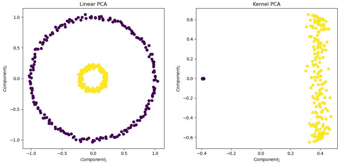
(2)使用核 PCA
核 PCA 是 PCA 的非线性扩展,当分类不是线性可分的,在进行 PCA 时通过核函数转换数据点,将数据映射到核空间,最后在核空间进行线性 PCA。
1
2
3
4
5
6
7
8
9
10
11
12
13
14
15
16
17
18
19
20
21
22
23
24
25
26
27
28
29
30
31
from sklearn.datasets import make_circles
from sklearn.decomposition import PCA
from sklearn.decomposition import KernelPCA

# 使用 make_circles 生成一个非线性数据集
np.random.seed(0)
# 二维特征,先验二分类,非线性:
X, Y = make_circles(n_samples=400, factor=0.2, noise=0.02)

# 可视化结果
def visualization(X, Y, title):
    '''可视化前两个主成分(一共有几百个)'''
    plt.figure(figsize=(6,6))
    plt.title(title)
    plt.scatter(X[:,0], X[:,1], c=Y)
    plt.xlabel('$Component_1$'); plt.ylabel('$Component_2$')
    plt.show()

# PCA 函数集成了上一节中的拟合预测等运算

# 首先使用线性 PCA
pca = PCA(n_components=2)
pca.fit(X)
x_pca = pca.transform(X)
visualization(x_pca, Y, 'Linear PCA')

# 使用核 PCA(径向基核函数)
kpca = KernelPCA(kernel='rbf', gamma=10)
kpca.fit(X)
x_kpca = kpca.transform(X)
visualization(x_kpca, Y, 'Kernel PCA')
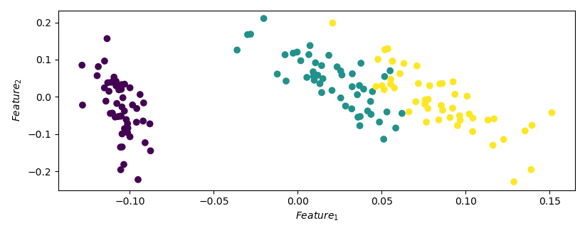
(3)使用奇异值分解提取特征
奇异值分解(Singular Value Decomposition, SVD):将一系列相关变量转换成不相关的变量,实现降维。SVD 常用于文本挖掘,用来挖掘语义关联。
和 PCA 不同,SVD 直接作用于原始数据矩阵,用较低维度的数据得到原始数据的最佳近似。本质上 SVD 不是一种机器学习方法,而是一种矩阵分解技术。公式表示为:$A=U*S*V^T$,其中 $U$、$V$ 分别称为“左、右奇异向量”,$S$ 为奇异值。
1
2
3
4
5
6
7
8
9
10
11
12
13
14
15
16
17
18
19
20
import scipy
from sklearn.datasets import load_iris
from sklearn.preprocessing import scale

# Load dataset
iris = load_iris()
X, Y = iris['data'], iris['target']
# Standardize(如果所有变量度量单位一致,可以不必进行缩放,只需中心化)
x_s = scale(X, with_mean=True, with_std=False, axis=0)

# 通过 SVD 提取特征
U, S, V = svd(x_s, full_matrices=False)
# 选用前两个奇异向量表示原始数据矩阵
x_t = U[:, :2]

# 可视化降维后的数据集
plt.figure(figsize=(5,5))
plt.scatter(x_t[:,0], x_t[:,1], c=Y)
plt.xlabel('$Feature_1$'); plt.ylabel('$Feature_2$')
plt.show()
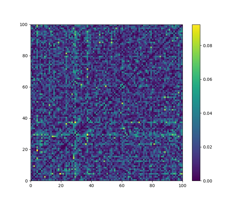
(4)用随机映射进行数据降维
PCA 和 SVD 的运算代价高昂,随机映射方法运算速度更快。根据 Johnson-Linden Strauss 定理的推论,从高维到低维的 Euclidean Space 的映射是存在的,可以使点到点的距离保持在一个 epsilon 的方差内。随机映射的目的就是保持任意两点之间的距离,同时降低数据的维度。
1
2
3
4
5
6
7
8
9
10
11
12
13
14
15
16
17
18
19
20
21
22
23
24
25
26
27
28
29
30
31
32
from sklearn.metrics import euclidean_distances
from sklearn.datasets import fetch_20newsgroups
from sklearn.feature_extraction.text import TfidfVectorizer
from sklearn.random_projection import GaussianRandomProjection

# 处理 20 个新闻组的文本数据,采用高斯随机映射
# 高斯随机矩阵是从正态分布 N(0, 1000^-1) 中采样生成的,1000是结果的维度

# 使用 sci.crypt 分类,将文本数据转换为向量表示
data = fetch_20newsgroups(categories='sci.crypt')
# 下载完会本地化,储存进 sklearn 模块

# 从 data 中创建一个 词-文档 矩阵,词频作为值
vectorizer = TfidfVectorizer(use_idf=False)
vector = vectorizer.fit_transform(data.data)
print(f'The Dimension of Original Data: {vector.shape}')
# 使用随机映射降维到 1000 维
gauss_proj = GaussianRandomProjection(n_components=1000)
gauss_proj.fit(vector)
# 将原始数据转换到新的空间
vector_t = gauss_proj.transform(vector)
print(f'The Dimension of Transformed Data: {vector_t.shape}')
# 检验是否保持了数据点的距离
org_dist = euclidean_distances(vector)
red_dist = euclidean_distances(vector_t)
diff_dist = abs(org_dist - red_dist)

# 上面的 diff_dist 返回一个 n x n 方阵,绘制成热力图:
plt.figure(figsize=(8, 8))
plt.pcolor(diff_dist[0:100, 0:100])
plt.colorbar()
plt.show()
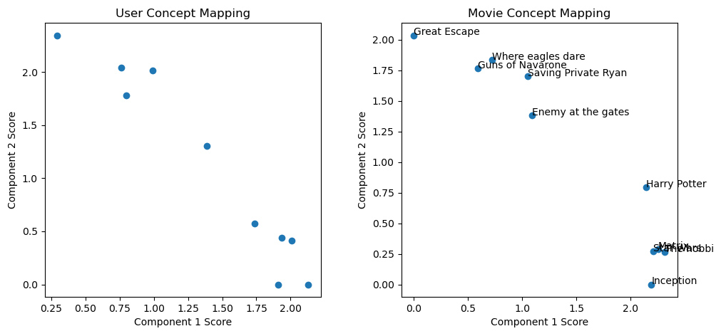
(5)使用 NMF 分解特征矩阵
前文使用主成分分析和矩阵分解技术进行降维,Non-negative Matrix Factorization(NMF)采用协同过滤算法进行降维。原理: 输入 $m*n$ 的矩阵 $A$,分解为 ${A_\bullet}(m*d)$ 和 $H(d*n)$,即:$A(m*n)={A_\bullet}*H$。约束条件:最小化 $|A-{A_\bullet}*H|^2$ 。
1
2
3
4
5
6
7
8
9
10
11
12
13
14
15
16
17
18
19
20
21
22
23
24
25
# 数据集:电影影评数据
ratings = [
    [5., 5., 4.5, 4.5, 5., 3., 2., 2., 0., 0.],
    [4.2, 4.7, 5., 3.7, 3.5, 0., 2.7, 2., 1.9, 0.],
    [2.5, 0., 3.3, 3.4, 2.2, 4.6, 4., 4.7, 4.2, 3.6],
    [3.8, 4.1, 4.6, 4.5, 4.7, 2.2, 3.5, 3., 2.2, 0.],
    [2.1, 2.6, 0., 2.1, 0., 3.8, 4.8, 4.1, 4.3, 4.7],
    [4.7, 4.5, 0., 4.4, 4.1, 3.5, 3.1, 3.4, 3.1, 2.5],
    [2.8, 2.4, 2.1, 3.3, 3.4, 3.8, 4.4, 4.9, 4.0, 4.3],
    [4.5, 4.7, 4.7, 4.5, 4.9, 0., 2.9, 2.9, 2.5, 2.1],
    [0., 3.3, 2.9, 3.6, 3.1, 4., 4.2, 0.0, 4.5, 4.6],
    [4.1, 3.6, 3.7, 4.6, 4., 2.6, 1.9, 3., 3.6, 0.]
]
movie_dict = {
    1: 'Star Wars',
    2: 'Matrix',
    3: 'Inception',
    4: 'Harry Potter',
    5: 'The hobbit',
    6: 'Guns of Navarone',
    7: 'Saving Private Ryan',
    8: 'Enemy at the gates',
    9: 'Where eagles dare',
    10: 'Great Escape'
}
1
2
3
4
5
6
7
8
9
10
11
12
13
14
15
16
17
18
19
20
21
22
23
24
25
26
27
28
29
from collections import defaultdict
from sklearn.decomposition import NMF

# 以下是模拟推荐系统的问题,通过用户对电影的评分,预测未知电影的评分。
A = np.asmatrix(ratings, dtype=float)
nmf = NMF(n_components=2, random_state=1)
A_dash = nmf.fit_transform(A)

# 检查降维后的矩阵
for i in range(A_dash.shape[0]):
    print(
        "User id = {}, comp_1 score = {}, comp_2 score = {}".format(
            i+1, A_dash[i][0], A_dash[i][1]
    ))
plt.figure(figsize=(5,5))
plt.title("User Concept Mapping")
plt.scatter(A_dash[:,0], A_dash[:,1])
plt.xlabel("Component 1 Score"); plt.ylabel("Component 2 Score")
plt.show()

# 检查成分矩阵
F = nmf.components_
plt.figure(figsize=(5,5))
plt.title("Movie Concept Mapping")
plt.scatter(F[0,:], F[1,:])
plt.xlabel("Component 1 Score"); plt.ylabel("Component 2 Score")
for i in range(F[0,:].shape[0]):
    plt.annotate(movie_dict[i+1], (F[0,:][i], F[1,:][i]))
plt.show()
第五章 数据挖掘
(1)使用距离度量
- 距离度量函数需要满足的条件:
- 输出是非负的
- 当且仅当 $X=Y$ 时输出为零
- 距离是对称的 $d(X, Y) = d(Y, X)$
- 遵循三角不等式:$d(X, Y) \geq{d(X, Z) + d(Z, Y)}$
- 常用度量方法:
- 欧氏距离:
- 欧几里得空间:空间中的点是由实数值组成的向量
- 欧几里得空间的点之间的物理距离成为欧氏距离,亦即 $l_2$ 范数:
- $d([x_1, x_2, …, x_n], [y_1, y_2, …, y_n]) = \sqrt{\sum_i{(x_i-y_i)^2}}$
- 余弦距离:
- 欧几里得空间,以及由整数或布尔值组成的向量空间,都可应用余弦距离
- 用两个向量夹角的余弦值度量
- 表达式:$X\cdot{Y} / \sqrt{X\cdot{X} * Y\cdot{Y}}$
- Jaccard 距离:
- 给定输入向量的集合,他们交集和并集的大小之比称为 Jaccard 系数,1 减去 Jaccard 系数即为 Jaccard 距离
- Hamming 距离:
- 对于两个位类型的数据,汉明距离就是这两个两个向量之间不同的位的数量
- Manhattan 距离:
- 又称 City Block Distance,也就是用 $l_1$ 范数度量的距离
- 欧氏距离:
1
2
3
4
5
euclidean_distance = lambda x, y: np.sqrt(np.sum(np.power((x-y), 2)))
LrNorm_distance = lambda x, y, r: np.power(np.sum(np.power((x-y), 2)), 1/r)
cosine_distance = lambda x, y: np.dot(x,y) / np.sqrt(np.dot(x,x) * np.dot(y,y))
jaccard_distance = lambda x, y: 1 - len(set(x).intersection(set(y))) / len(set(x).union(set(y)))
hamming_distance = lambda x, y: sum([i != j for i, j in zip(x, y)])
(2)使用核函数
当数据非线性时,要使用线性模型,需要进行复杂的运算进行线性化。使用核函数可以更便捷地处理非线性数据。核函数的数学定义:$k(X_i, j_i) = \phi(X_i)\cdot\phi(X_j)$。这里的 $X_i$ 和 $X_j$ 为输入向量,映射函数 $\phi(\cdot)$ 将输入向量映射到一个新的空间。
例如设定映射函数为 $\phi(X_1, X_2, X_3) = (X_1^2, X_2^2, X_3^2, X_1{X_2}, X_1{X_3}, X_2{X_3}, X_3,X_2,X_1)$,就可以将输入变量映射到新的空间。
1
2
3
4
5
6
7
8
9
10
11
12
13
14
15
16
17
18
# 示例:在三维数据上简单应用核函数
x = np.array([10, 20, 30])
y = np.array([8, 9, 10])

# 定义核函数:
def mapping_function(x):
    output_list = []
    for i in range(len(x)):
        for j in range(len(x)):
            output_list.append(x[i]*x[j])
    return np.array(output_list)

# 应用核函数
x_t = mapping_function(x)
y_t = mapping_function(y)
print(x_t)
print(y_t)
print(np.dot(x_t, y_t))
(3)K Means 聚类
K Means 聚类原理参考 R 统计学习笔记。
1
2
3
4
5
6
7
8
9
10
11
12
13
14
15
16
17
18
19
20
from sklearn.cluster import KMeans
from sklearn.metrics import silhouette_score

# 随机数据
x_1 = np.random.normal(loc=0.2, scale=0.2, size=(100, 100))
x_2 = np.random.normal(loc=0.9, scale=0.1, size=(100, 100))
x = np.r_[x_1, x_2]

# 将不同 K 值的聚类打包成函数
def form_clusters(x, k):
    km = KMeans(n_cluster=k, init='random')
    km.fit(x)
    return silhouette_score(x, km.labels_)

# 进行参数选择
silh_scores = []
for i in range(10):
    ss = form_clusters(x, i+2)
    silh_scores.append(ss)
# 当 K=2 时轮廓系数最大,聚类最好
(4)学习向量量化
Learning Vector Quantization(LVQ)是一种无模型数据点聚类方法。与其他方法不同,它无法解释响应变量和预测变量直接的关系。在实际应用中,作为黑箱方法应用。
LVQ 是一种在线学习方法,每次只处理一个数据点。步骤如下:
- 为数据集里的每个类型选择 K 个原型向量。例如对于二分类问题,每个分类选择两个原型向量,则需要设置 4 个原型向量。它们从数据集中随机地选取;
- 接着确定一个 epsilon 值,进行循环,直到 epsilon 变为 0 或预设的阈值;
- 在上述的每次循环中,都采样一个输入点,采用欧氏距离找出其最近的原型向量。
1
2
3
4
5
6
7
8
9
10
11
12
13
14
15
16
17
18
19
20
21
22
23
24
25
26
27
28
29
30
31
32
33
34
35
36
37
38
39
40
41
42
43
44
45
46
47
48
49
50
51
52
53
54
55
56
57
58
59
60
61
62
63
64
65
66
67
68
69
70
71
72
73
74
75
76
77
78
79
80
81
82
83
84
85
86
87
88
from sklearn.datasets import load_iris
from sklearn.preprocessing import MinMaxScaler
from sklearn.metrics import classification_report
#from sklearn.metrics.pairwise import euclidean_distances

euclidean_distance = lambda x, y: np.sqrt(np.sum(np.power((x-y), 2)))

# 定义一个类来保存原型向量
class Prototype(object):

    def __init__(self, class_id, p_vector, epsilon):
        self.class_id = class_id
        self.p_vector = p_vector
        self.epsilon = epsilon

    def update(self, u_vector, increment=True):
        step = self.epsilon * (u_vector - self.p_vector)
        if increment:
            # 将原型向量靠近输入向量
            self.p_vector = self.p_vector + step
        else:
            # 将原型向量远离输入向量
            self.p_vector = self.p_vector - step

# 寻找离给定向量最近的原型向量
def find_closest(in_vector, proto_vectors):
    closest = None
    closest_distance = 1e5
    for p_v in proto_vectors:
        distance = euclidean_distance(in_vector, p_v.p_vector)
        if distance < closest_distance:
            closest_distance = distance
            closest = p_v
    return closest

# 找出最近的原型向量的类别ID
find_class_id = lambda vec, vecs: find_closest(vec, vecs).class_id

# if __name__ == "__main__":
# Loading dataset
iris = load_iris()
X = iris['data']; Y = iris['target']

# 最小最大缩放
minmax = MinMaxScaler()
x = minmax.fit_transform(X)

# 为每个类选择R个原型向量
p_vectors = []
for i in range(3):
    x_subset = x[np.where(Y==i)]
    # 获取R个随机下标,介于0-50
    samples = np.random.randint(0, len(x_subset), 2)
    # 选择原型向量
    for sample in samples:
        s = x_subset[sample]
        p = Prototype(i, s, epsilon=0.9)
        p_vectors.append(p)
print("class id | Initial prototype vector")
for p_v in p_vectors:
    print(p_v.class_id, '\t\t |', p_v.p_vector)

# 利用已有的数据点,执行循环调整原型向量,对新的点进行分类
epsilon = 0.9; delta_epsilon = 0.001
while epsilon >= 0.01:
    # 随机采样一个训练实例
    rnd_i = np.random.randint(0, 149)
    rnd_s = x[rnd_i]
    target_y = Y[rnd_i]
    # 为下一次循环减少epsilon
    epsilon = epsilon - delta_epsilon
    # 查找与给定点最近的原型向量
    closest_pvector = find_closest(rnd_s, p_vectors)
    # 更新最近的原型向量
    if target_y == closest_pvector.class_id:
        closest_pvector.update(rnd_s)
    else:
        closest_pvector.update(rnd_s, False)
    closest_pvector.epsilon = epsilon
print("class_id | Final Prototype Vector")
for p_v in p_vectors:
    print(p_v.class_id, '\t\t |', p_v.p_vector)

# 把原型向量用于预测
y_pred = [find_class_id(instance, p_vectors) for instance in X]
# 根据上面获得的原型向量预测类别
print(classification_report(Y, y_pred,
        target_names=['Setosa', 'Verssicolour','Virginaca']))
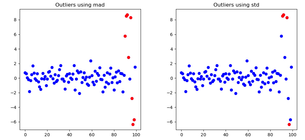
(5)在单变量数据中找出异常点
在单变量中寻找异常数据的几种常用方法:
- 绝对中位差
- 平均值加或减去 3 倍标准差
1
2
3
4
5
6
7
8
9
10
11
12
13
14
15
16
17
18
19
# 创建100个数据点,其中10%是outliers/
n_samples = 100
fraction_of_outliers = 0.1
number_outliers = int(fraction_of_outliers * n_samples)
number_inliers = n_samples - number_outliers

# 创建数据
normal_data = np.random.randn(number_inliers, 1)
print(" | Mean: %0.2f | Standard Deviation: %0.2f |"\
        % (np.mean(normal_data), np.std(normal_data)))
outlier_data = np.random.uniform(low=-9, high=9, size=(number_outliers, 1))
data = np.r_[normal_data, outlier_data]
print(f"Shape of total data: {data.shape}")

# 显示数据
plt.figure(figsize=(5, 5))
plt.title("Input Data Points")
plt.scatter(range(len(data)), data, c='b')
plt.show()
1
2
3
4
5
6
7
8
9
10
11
12
13
14
15
16
17
18
19
20
21
22
23
24
25
26
27
28
29
30
31
32
33
34
35
36
37
38
39
'''
mad 对应绝对中卫差方法,std 对应 3 倍标准差方法
'''
def show_result(data, method):

    mean = np.mean(data)
    std = np.std(data)
    median = np.median(data)

    # 定义上限和下限
    if method == 'mad':
        b = 1.4826
        mad = b * np.median(np.abs(data - median))
        lower_limit = median - 3 * mad
        upper_limit = median + 3 * mad
    elif method == 'std':
        b = 3
        lower_limit = mean - b * std
        upper_limit = mean + b * std

    # 寻找outliers
    outliers = []
    outliers_index = []
    for i in range(len(data)):
        if data[i] > upper_limit or data[i] < lower_limit:
            outliers.append(data[i])
            outliers_index.append(i)

    # 绘图显示异常点
    plt.figure(figsize=(5,5))
    plt.title(f"Outliers using {method}")
    plt.scatter(range(len(data)), data, c='b')
    plt.scatter(outliers_index, outliers, c='r')
    plt.show()

show_result(data, method='mad')
show_result(data, method='std')

# 可见使用中位值作为评估值比使用均值更加健壮,不容易干扰。
(6)使用局部异常因子方法发现异常点
Local Outlier Factor(LOF)对数据的局部密度和邻居进行比较,判断这个数据点是否属于相似的密度区域。适用簇的个数未知,簇的密度和大小各不相同的数据中筛选异常点。这种算法思想源自 KNN。
相关术语:
- 对象 P 的 K 距离:对象 P 与其第 K 个最邻近的点的距离,K为自由参数
- P 的 K 距离邻居:距离小于或等于 P 的 K 距离的对象的集合 Q
- P 到 Q 的可达距离(reachability distance):P 与 其第 K 个最近邻的距离,和 P 与 Q 之间的距离,两者之间的最大值
- P 的局部可达密度(Local Reachability Density, LRD):K 距离邻居和 K 与其邻居的可达距离之和的比值
- P 的局部异常因子(LOF):P 与它的 K 最近邻的局部可达距离的比值的平均值
1
2
3
4
5
6
7
8
9
10
11
12
13
14
15
16
17
18
19
20
21
22
23
24
25
26
27
28
29
30
31
32
33
34
35
36
37
38
39
40
41
42
43
44
45
46
47
48
49
50
51
52
53
54
55
56
57
58
59
60
61
62
63
64
65
66
67
68
69
70
71
72
73
74
import headq
from collections import defaultdict
from sklearn.metrics import pairwise_distances

# generate data
instances = np.matrix([[0,0], [0,1], [1,1], [1,0], [5,0]])
x = np.squeeze(np.array(instances[:,0]))
y = np.squeeze(np.array(instances[:,1]))

'''计算两两之间的距离'''
k = 2
dist = pairwise_distances(instances, metric='manhattan')

'''计算K距离'''
k_distance = defaultdict(tuple)
for i in range(instances.shape[0]):
    # 获得当前点与其他各点之间的距离
    distances = dist[i].tolist()
    # 获得K最近邻及其索引
    kneighbors = heapq.nsmallest(k+1, distances)[1:][k-1]
    neighbors_idx = distances.index(kneighbors)
    # 每个点的第K个最近邻以及距离
    k_distance[i] = (kneighbors, neighbors_idx)

'''计算K距离邻居'''
def all_indices(value, inlist):
    out_indices = []
    idx = -1
    while True:
        try:
            idx = inlist.index(value, idx+1)
            out_indices.append(idx)
        except ValueError:
            break
    return out_indices

k_distance_neig = defaultdict(list)
for i in range(instances.shape[0]):
    distances = dist[i].tolist()
    print("k distance neighbourhood", i)
    print(distances)
    # 获取 1-K 最邻近
    kneighbors = heapq.nsmallest(k+1, distances)[1:]
    print(kneighbors)
    print(set(kneighbors))

    kneighbors_idx = []
    # 获取 K 里最小的元素的索引
    for x in set(kneighbors):
        kneighbors_idx.append(all_indices(x, distances))
    # 将 列表列表 转化为 列表
    kneighbors_idx = [item for sublist in kneighbors_idx for item in sublist]
    # 对每个点保存其k距离邻居
    k_distance_neig[i].extend(zip(kneighbors, kneighbors_idx))

'''计算可达距离和局部可达密度LRD'''
lrd = defaultdict(float)
for i in range(instances.shape[0]):
    # LRD的分子,也就是K距离邻居的个数
    no_neighbors = len(k_distance_neig[i])
    # 可达距离求和作为分母
    denom_sum = 0
    for neigh in k_distance_neig[i]:
        denom_sum += max(k_distance[neigh[1]][0], neigh[0])
    lrd[i] = no_neighbors / (1. * denom_sum)

'''计算LOF'''
lof_list = []
for i in range(instances.shape[0]):
    lrd_sum, rdist_sum = 0, 0
    for neigh in k_distance_neig[i]:
        lrd_sum += lrd[neigh[1]]
        rdist_sum += max(k_distance[neigh[1]][0], neigh[0])
    lof_list.append((i, lrd_sum * rdist_sum))