第六章 机器学习(I)
(1)为建模准备数据
1
2
3
4
5
6
7
8
9
10
11
12
13
14
15
16
17
18
19
20
21
22
23
24
25
26
27
28
29
30
31
from sklearn.datasets import load_iris
from sklearn.model_selection import train_test_split

X, y = load_iris()['data'], load_iris()['target']
# 将 Features 和 Target 合并
input_data = np.column_stack([X, y])
# 洗乱数据
data = np.random.shuffle(input_data)

# 分集
x_train, x_test, y_train, y_test = train_test_split(X, y, test_size=0.3)

# 检验训练集和测试集是否存在类别标签分布不平衡
def get_class_distribution(y):
    distribution = {}
    for label in set(y):
        distribution[label] = len(np.where(y==label)[0])
    distribution_pct = {
        label: count/sum(distribution.values())
        for label, count in distribution.items()
    }
    return distribution_pct

train_distribution = get_class_distribution(y_train)
test_distribution = get_class_distribution(y_test)
print("\nTrain dataset class label distribution\n" + '='*66)
for k,v in train_distribution.items():
    print(f"class label: {k:d}, percentage: {v:0.2f}")
print("\nTest dataset class label distribution\n" + '=' * 66)
for k,v in test_distribution.items():
    print(f"class label: {k:d}, percentage: {v:0.2f}")
(2)最邻近算法
衡量分类结果好坏的指标:
- 混淆矩阵:label的真实值和预测值的排列矩阵,可以用 pandas 层次化DataFrame表示:
1
2
3
4
5
6
7
confusion_matrix = pd.DataFrame(
    [['TP','FN'], ['FP','TN']],
    columns=pd.MultiIndex.from_tuples(
        [('Prediction','T'),('Prediction','F')]),
    index=pd.MultiIndex.from_tuples(
        [('Ground Truth','T'),('Ground Truth','F')])
    )
| (‘Prediction’, ‘T’) | (‘Prediction’, ‘F’) | |
|---|---|---|
| (‘Ground Truth’, ‘T’) | TP | FN |
| (‘Ground Truth’, ‘F’) | FP | TN |
- 准确度:Accuracy = Correct_Prediction / Total_Prediction;其中:Correct_Prediction = TP + TN
- 另外还有错误率等其他指标
K Nearest Neighborhood, KNN
- 机械分类算法:把所有的训练数据加载到内存,当需要预测一个未知的实例时,在内存里比对所有的训练实例,匹配每一个属性来确定分类标签
- 上述算法中,如果找不到完全匹配的实例,就无法分配标签。KNN 可以理解为它的改进,不进行完全匹配,而是采用相似度量。
- 具体来说,KNN 在预测时,计算待预测实例与所有训练数据的距离,选择 K 个最近的实例,基于这K个最近邻的主体分类,对未知实例进行预测
1
2
3
4
5
6
7
8
9
10
11
12
13
14
15
16
17
18
19
20
21
22
23
24
25
26
27
28
29
30
31
32
33
34
35
36
37
38
import itertools
from sklearn.datasets import make_classification
from sklearn.metrics import classification_report
from sklearn.ensemble import BaggingClassifier
from sklearn.neighbors import KNeighborsClassifier
from sklearn.model_selection import StratifiedShuffleSplit
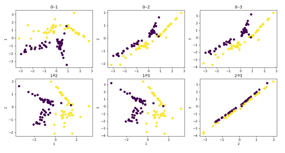
def show_data(X, y):
'''可视化数据集'''
# 生成迭代器:[0,1,2,3] 的二元组合数
col_pairs = itertools.combinations(range(4), 2)
subplots = 231
plt.figure(figsize=(8,9), dpi=80)#, facecolor='#999999')
# 绘制每个特征两两组合的散点图
for pair in col_pairs:
plt.subplot(subplots)
plt.scatter(X[:,pair[0]], X[:,pair[1]], c=y)
plt.title(str(pair[0]) + '--' + str(pair[1]))
plt.xlabel(str(pair[0])); plt.ylabel(str(pair[1]))
subplots += 1
plt.show()
def split_data(x, y):
'''prepare a stratified train and test split'''
sss = StratifiedShuffleSplit(test_size=0.2, n_splits=1)
# 默认n_splits=10,也就是下面for循环会执行10次,但只保存了最后一次的值
# 必须使用for循环,因为 StratifiedShuffleSplit 是惰性的生成器
for train_idx, test_idx in sss.split(x, y):
train_x = X[train_idx]
train_y = y[train_idx]
test_x = X[test_idx]
test_y = y[test_idx]
return train_x, train_y, test_x, test_y
# if __name__ == "__main__":
# 生成虚拟分类数据并可视化
X, y = make_classification(n_features=4)
show_data(X, y) # 可见各个变量之间都存在多重线性关系
1
2
3
4
5
6
7
8
9
10
11
12
13
14
15
16
17
# 生成分层的训练集和测试集,使训练集和测试集的标签分布一致
x_train, y_train, x_test, y_test = split_data(X, y)

# build and fit model
knn = KNeighborsClassifier(n_neighbors=2)
knn.fit(x_train, y_train)
# 查看模型参数
print(knn.get_params())

# predict and evaluate model
print("\nModel evaluation on training set\n" + '='*66)
y_train_pred = knn.predict(x_train)
print(classification_report(y_train, y_train_pred))

print("\nModel evaluation on test set\n" + '='*66)
y_test_pred = knn.predict(x_test)
print(classification_report(y_test, y_test_pred))
(3)朴素贝叶斯分类
- 贝叶斯公式:P(X|Y) = P(Y|X) * P(X) / P(Y),即已知事件 Y 发生时,事件 X 发生的条件概率
- 常用于自然语言处理算法
- nltk:python 自然语言处理库
(4)构建决策树解决多分类问题
- 关于决策树的基础知识参考“R 统计学习笔记”
- 一些提高效率,短时间生成较合理的决策树的算法:
- Hunt
- ID3
- C4.5
- CART
- target 的属性种类:
- 二元属性
- 标称属性(n 个值)
- 序数属性(如:小中大)
- 连续属性(连续变量离散化形成)
- 决策树的不足:
- 容易过拟合
- 给定一个数据集,能产生巨量的决策树
- 对类别不平衡敏感
1
2
3
4
5
6
7
8
9
10
11
12
13
14
15
16
17
18
19
20
21
22
23
24
25
26
27
28
29
30
31
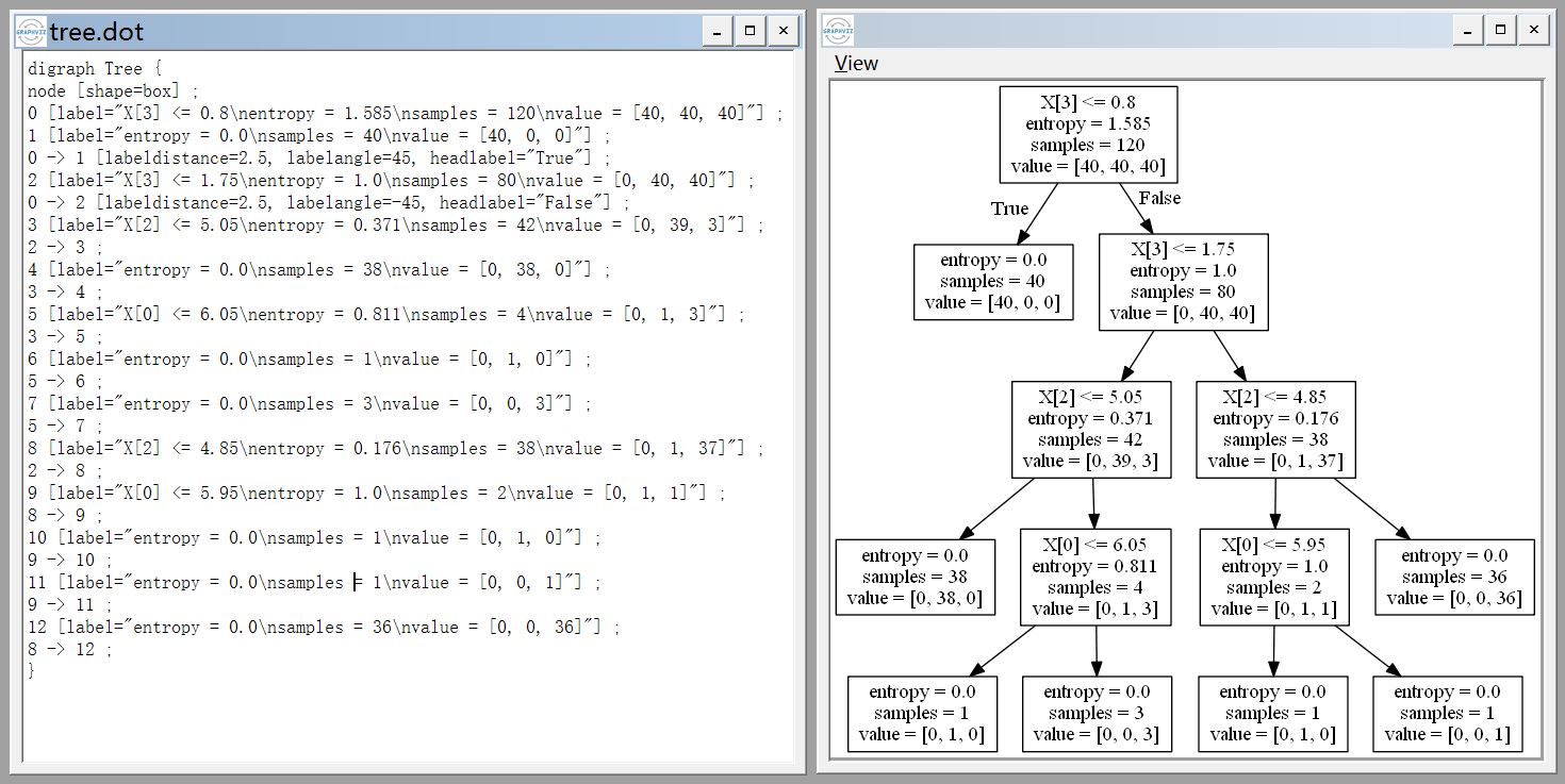
from pprint import pprint
from sklearn.datasets import load_iris
from sklearn.model_selection import StratifiedShuffleSplit
from sklearn.metrics import accuracy_score, confusion_matrix
from sklearn.metrics import classification_report
from sklearn.tree import DecisionTreeClassifier, export_graphviz
def split_data(X, y):
sss = StratifiedShuffleSplit(test_size=0.2, n_splits=1)
for train_idx, test_idx in sss.split(X, y):
x_train = X[train_idx]; x_test = X[test_idx]
y_train = y[train_idx]; y_test = y[test_idx]
return x_train, x_test, y_train, y_test
if __name__ == "__main__":
X, y = load_iris()['data'], load_iris()['target']
label_names = load_iris()['target_names']
x_train, x_test, y_train, y_test = split_data(X, y)
dtree = DecisionTreeClassifier(criterion='entropy') #熵判断准则
dtree.fit(x_train, y_train)
# evaluation
y_pred = dtree.predict(x_test)
print("Model accuracy = {:0.4f}".format(accuracy_score(y_test, y_pred)))
print("\nConfusion Matrix:\n" + '='*66)
print(pprint(confusion_matrix(y_test, y_pred)))
print("\nClassification Report:\n" + '='*66)
print(classification_report(y_test, y_pred, target_names=label_names))
# 导出树图(.dot 文件可以安装 graphviz 后使用 gvedit.exe 打开)
export_graphviz(dtree, out_file='tree.dot')
第七章 机器学习(II)
(1)回归方法预测实数值
1
2
3
4
5
6
7
8
9
10
11
12
13
14
15
16
17
18
19
20
21
22
23
24
25
26
27
28
29
30
31
32
33
34
35
36
37
38
39
40
41
42
43
44
45
46
47
48
49
50
51
52
53
54
55
56
57
58
59
60
61
62
63
64
65
66
67
68
69
70
71
# coding = utf-8
""" 一个简单的OLS线性回归例子,使用Boston数据集。
"""
import matplotlib.pyplot as plt
from itertools import combinations
from sklearn.datasets import load_boston
from sklearn.model_selection import train_test_split
from sklearn.feature_selection import RFE
from sklearn.metrics import mean_squared_error
from sklearn.linear_model import LinearRegression
from sklearn.preprocessing import PolynomialFeatures

def split_data(x, y, train_size, test_size, seed=1):
    x_train, x_temp, y_train, y_temp = \
        train_test_split(x, y, test_size=1-train_size, random_state=seed)
    size = test_size / (1 - train_size)
    x_dev, x_test, y_dev, y_test = \
        train_test_split(x_temp, y_temp, test_size=size, random_state=seed)
    return x_train, x_dev, x_test, y_train, y_dev, y_test

def plot_residual(model, x_train, y_train):
    prediction = model.predict(x_train)
    plt.figure(figsize=(8,9), dpi=80)
    plt.title("Residual Plot")
    plt.plot(prediction, y_train - prediction, 'go')
    plt.xlabel("Prediction"); plt.ylabel("Residual")
    plt.show()

def view_model(model, y, y_hat):
    print("\nModel Coefficients:\n" + '='*66)
    for i, coef in enumerate(model.coef_):
        print(f"\tCoefficient_{i+1:d}: {coef:0.2f}")
    print(f"\tIntercept: {model.intercept_:0.3f}")
    print("Mean Squared Error: {:0.2f}".format(mean_squared_error(y, y_hat)))

if __name__ == "__main__":
    '''最小二乘线性回归'''
    X, y = load_boston()['data'], load_boston()['target']
    x_train, x_dev, x_test, y_train, y_dev, y_test = split_data(X, y, 1/3, 1/3)
    lm = LinearRegression(normalize=True, fit_intercept=True)
    lm.fit(x_train, y_train)
    # 绘制残差
    plot_residual(lm, x_train, y_train)
    # 查看模型参数
    view_model(lm, y_train, lm.predict(x_train))
    # 验证集MSE
    print(mean_squared_error(y_dev, lm.predict(x_dev)))

    '''使用多项式特征'''
    polyfeat = PolynomialFeatures(degree=2, interaction_only=False)
    polyfeat.fit(x_train)
    x_train_poly = polyfeat.transform(x_train)
    x_dev_poly = polyfeat.transform(x_dev)
    poly_lm = LinearRegression(normalize=True, fit_intercept=True)
    poly_lm.fit(x_train_poly, y_train)
    plot_residual(poly_lm, x_train_poly, y_train)
    view_model(poly_lm, y_train, poly_lm.predict(x_train_poly))
    print(mean_squared_error(y_dev, poly_lm.predict(x_dev_poly)))

    '''递归特征选择方法--线性回归的低偏差高反差问题,也就是测试集误差大。'''
    # generate polynomial features
    polyfeat = PolynomialFeatures(interaction_only=True)
    polyfeat.fit(x_train)
    x_train_poly = polyfeat.transform(x_train)
    x_dev_poly = polyfeat.transform(x_dev)
    # build model
    lm = LinearRegression(normalize=True, fit_intercept=True)
    rfe_lm = RFE(estimator=lm, n_features_to_select=20)
    rfe_lm.fit(x_train_poly, y_train)
    # evaluate model
    plot_residual(rfe_lm, x_train_poly, y_train)
(2)岭回归
1
2
3
4
5
6
7
8
9
10
11
12
13
14
15
16
17
18
19
20
21
22
23
24
25
26
27
28
29
30
31
32
33
34
35
36
37
38
39
40
41
42
43
44
45
46
47
48
49
50
51
52
53
54
55
56
57
58
59
60
# coding = utf-8
""" 主要功能:在OLS回归中加入惩罚项,以限制权重参数的大小;详细参考ISLR。
"""
import numpy as np
import matplotlib.pyplot as plt
from sklearn.datasets import load_boston
from sklearn.linear_model import Ridge
from sklearn.metrics import mean_squared_error
from sklearn.model_selection import train_test_split
from sklearn.preprocessing import PolynomialFeatures

def split_data(x, y, train_size, test_size, seed=1):
    x_train, x_temp, y_train, y_temp = \
        train_test_split(x, y, test_size=1-train_size, random_state=seed)
    size = test_size / (1 - train_size)
    x_dev, x_test, y_dev, y_test = \
        train_test_split(x_temp, y_temp, test_size=size, random_state=seed)
    return x_train, x_dev, x_test, y_train, y_dev, y_test


if __name__ == "__main__":
    # load data
    X, y = load_boston()['data'], load_boston()['target']
    X = X - np.mean(X, axis=0)
    x_train, x_dev, x_test, y_train, y_dev, y_test = split_data(X, y, 2/3, 1/9)

    # generate polynomial features
    polyfeat = PolynomialFeatures(interaction_only=True)
    polyfeat.fit(x_train)
    for name in ['train', 'dev', 'test']:
        exec(f"x_{name}_poly = polyfeat.transform(x_{name})")

    # build, fit and evaluate model
    rm = Ridge(normalize=True, alpha=0.015)
    rm.fit(x_train_poly, y_train)
    y_pred = rm.predict(x_train_poly)
    mse = mean_squared_error(y_train, y_pred)
    print("\nModel coefficients: \n" + '='*66)
    for i, coef in enumerate(rm.coef_):
        print(f"\tCoefficient_{i+1:d}:\t{coef:0.3f}")
    print(f"Intercept: {rm.intercept_}")

    # repeat above on dev and test split ...

    # 向X中加入噪音,测试模型敏感性(非常敏感)
    # X = X + np.random.normal(0, 1, (X.shape))

    # 参数查找
    alphas = np.linspace(10, 100, 300)    # [10 - 100], length=300
    coefficients = []
    for a in alphas:
        model = Ridge(normalize=True, alpha=a)
        model.fit(X, y)
        coefficients.append(model.coef_)
    # 绘制每个参数(共13个)随着alpha的变化
    plt.figure(figsize=(6,6.75), dpi=80)
    plt.title("Coefficient Weights for Different Alpha Values")
    plt.plot(alphas, coefficients)
    plt.xlabel("Alpha"); plt.ylabel("Weight")
    plt.show()
(3)lasso
1
2
3
4
5
6
7
8
9
10
11
12
13
14
15
16
17
18
19
20
21
22
23
24
25
26
27
28
29
30
31
32
33
34
35
36
37
38
39
40
41
42
43
44
# coding = utf-8
""" 与岭回归相比,Lasso可以筛选参数,具有稀疏特性,详细参考ISLR。
"""
import numpy as np
import matplotlib.pyplot as plt
from sklearn.datasets import load_boston
from sklearn.metrics import mean_squared_error
from sklearn.model_selection import train_test_split
from sklearn.preprocessing import PolynomialFeatures
from sklearn.linear_model import Lasso, LinearRegression

# load data
X, y = load_boston()['data'], load_boston()['target']

# build models on parameters grid and get coefficients
alphas = np.linspace(0, 0.5, 200)
model = Lasso(normalize=True)
coefficients = []
for alpha in alphas:
    model.set_params(alpha=alpha)
    model.fit(X, y)
    coefficients.append(model.coef_)

# 绘制权重随着参数的变化
plt.figure(figsize=(6,6.75), dpi=80)
plt.title("Coefficient Weights for Different Alpha Values")
plt.plot(alphas, coefficients)
plt.vlines(x=0.1, ymin=-2, ymax=5, color='r', alpha=0.1)
plt.xlabel("Alpha"); plt.ylabel("Weight")
plt.axis('tight')
plt.show()

# 根据上面的图示选择合适参数,暂定选择alpha=0.1,保留4个变量
model = Lasso(normalize=True, alpha=0.1)
model.fit(X, y)
# 也可以使用mse作为criterion递归查找最优参数

# 模型参数和MSE(训练集误差)
print("\nModel Coefficients: \n" + '='*66)
for i, coef in enumerate(model.coef_):
    print(f"\tCoefficient_{i+1:d}:\t{coef:0.3f}")
print(f"Intercept: {model.intercept_}")
print("MSE: {:0.3f}".format(mean_squared_error(y, model.predict(X))))
(4)L1 缩减和 L2 缩减交叉验证
1
2
3
4
5
6
7
8
9
10
11
12
13
14
15
16
17
18
19
20
21
22
23
24
25
26
27
28
29
30
31
32
33
34
35
36
37
38
39
40
41
42
43
44
45
# coding = utf-8
""" ·现实场景中,数据集一般不够大,可以通过交叉验证进行模型选择。详细参考ISLR。
    ·交叉验证迭代器的使用参考documentation的examples
    ·以下对lasso回归模型进行交叉验证。
"""
import numpy as np
from sklearn.linear_model import Ridge
from sklearn.datasets import load_boston
from sklearn.metrics import mean_squared_error
from sklearn.preprocessing import PolynomialFeatures
from sklearn.model_selection import KFold, train_test_split, GridSearchCV

# load and split data
X, y = load_boston()['data'], load_boston()['target']
x_train, x_test, y_train, y_test = train_test_split(X, y,
                                    test_size=0.3, random_state=0)
# generate polynomial features
polyfeat = PolynomialFeatures(interaction_only=True)
polyfeat.fit(x_train)
for name in ['train', 'test']:
    exec(f"x_{name}_poly = polyfeat.transform(x_{name})")

# build model
rr = Ridge(normalize=True)
kfold = KFold(n_splits=5)
param_grid = {'alpha': np.linspace(0.0015, 0.0017, 30)}
grid = GridSearchCV(estimator=rr,
                    param_grid=param_grid,
                    cv=kfold,
                    scoring='neg_mean_squared_error')
# 调用fit实例方法,将在定义的参数范围内,进行k折交叉验证
grid.fit(x_train_poly, y_train)

# 查看不同参数的结果
print(grid.cv_results_)
print(grid.best_params_)
# 保存最佳模型
best_model = grid.best_estimator_
print(best_model.coef_)
# 计算最佳模型的测试集MSE
mse = mean_squared_error(y_train, best_model.predict(x_train_poly))

'''
关于GridSearchCV对象的更多属性和方法以及其他交叉验证器请参考scikit-learn文档。
'''