第八章 集成方法
集成学习(Ensemble Learning)的概念:不仅仅通过个人,而是通过集体智慧来做出决策。准确来说,就是生成大量模型,用它们来进行预测。从多个相近的模型输出的结果会比仅仅从一个模型的到的结果更好。集成的模型可以是不同类别的,比如同时利用神经网络模型和贝叶斯模型。本章只讨论集成同类的模型。
挂袋法,每个模型只使用训练集的一部分,以减少过拟合。挂袋法很容易实现并行化,可以同时处理的不同的训练集样本。挂袋法对如线性回归之类的线性预测器无效。
提升法,产生一个逐步复杂的模型序列,基于上一个模型的错误,训练新的模型。每次训练的模型被赋予一个权重,并按权重得出最终的预测值。可见提升法是按顺序执行的,无法并行化。提升法常常用一些弱分类器,如单层决策树。
(1)装袋法
集成方法属于基于评委学习方法一族。挂袋法也叫引导聚集,只有在潜在的模型能产生不同变化时才有效。也就是要产生有轻微变化的多种模型。
使用自举方法在模型上产生变化,自举就是在数据集中随机采样一定的观测,不管是否有替换。在挂袋法中,通过自举产生 m 个数据集,然后对每一个建立一个模型,最终使用所有模型的输出来产生最终的预测。对于回归问题就是取均值,对于分类问题使用投票方法。
挂袋法适用于不稳定的、对变化敏感的模型,例如决策树,尤其未剪枝的。而不适合 KNN 等稳定的分类器。应用于 KNN 时需要使用随机子空间方法(例如,在集成的每个模型里随机选择特征属性的子集)。
1
2
3
4
5
6
7
8
9
10
11
12
13
14
15
16
17
18
19
20
21
22
23
24
25
26
27
28
29
30
31
32
33
34
35
36
37
38
39
40
41
42
43
44
45
from sklearn.datasets import make_classification
from sklearn.model_selection import train_test_split
from sklearn.metrics import classification_report
from sklearn.neighbors import KNeighborsClassifier
from sklearn.ensemble import BaggingClassifier

# generate a dataset for classification
X, y = make_classification(n_samples=500, n_features=30, flip_y=0.03,
    n_informative=18, n_redundant=3, n_repeated=3, random_state=1)
# 一共30个特征,18个关键特征,3个多余的特征,3个重复的特征,flip_y使分类更困难

# split data
x_train, x_temp, y_train, y_temp = \
            train_test_split(X, y, test_size=0.3, random_state=1)
x_dev, x_test, y_dev, y_test = \
            train_test_split(x_temp, y_temp, test_size=0.3, random_state=1)

# generate a KNN classifier, then report
knn = KNeighborsClassifier()
knn.fit(x_train, y_train)
y_pred_knn = knn.predict(x_train)
print(classification_report(y_train, y_pred_knn))

# generate a Bagging classifier on KNN, then report
bagging = BaggingClassifier(KNeighborsClassifier(), n_estimators=100,
                            max_samples=1.0, max_features=0.7,
                            bootstrap=True, bootstrap_features=True,
                            random_state=1)
# estimator自举时选用100%的样本,选取70%的特征属性(随机空间方法)
# 样本与特征的采样都是有放回(default=False)
bagging.fit(x_train, y_train)
y_pred_bagging = bagging.predict(x_train)
print(classification_report(y_train, y_pred_bagging))
# 可以看到bagging比knn的准确率明显提高

# 打印出前 3 个模型所选取的特征属性
print("\nSampled attributes in top 3 estimators: \n" + '='*66)
for i, features in enumerate(bagging.estimators_features_[0:3]):
    print(f"estimator_{i+1:d}: ", features)

# 在验证集上对比knn和bagging
print("\nSingle KNN: \n" + '='*66)
print(classification_report(y_dev, knn.predict(x_dev)))
print("\nBagging KNN: \n" + '='*66)
print(classification_report(y_dev, bagging.predict(x_dev)))
(2)提升法
a) Boosting 原理步骤:
对于二分类问题,分类器的输入可以表达为:$X = [x_1, x_2, …, x_N]\ and\ Y = [0, 1]$。 分类器的任务就是找到一个可以近似的函数:$Y = F(X)$。
分类器的错误率定义为:$error\ rate = \frac{1}{N} * \sum_i{[instance\ |\ y_i \neq{F(x_i)}]}$
假设构建一个弱分类器(错误率仅好于随机猜测),然后通过提升法构建一系列弱分类器用在经过微调的数据集上,每个分类器使用的数据只做了很小的调整。最后结束于第 $M$ 个分类器:$F_1(X), F_2(X), …, F_M(X)$
最后把各个分类器生成的预测集成起来,进行加权投票:$F_{final}(X) = sign( \sum_i(\alpha_i * F_i(X)) )$,其中 $\alpha_i$ 为模型 $F_i(\cdot)$ 的权重。
b) 模型权重计算原理步骤:
首先修改错误率公式:$error\ rate = \sum_i( w_i * |y_i - \hat{y_i}| ) / \sum_i( w_i )$
对于 $N$ 个实例,每个实例的权重为 $1/N$ ,$w_i$ 表示模型的初始权重 $w_i = n / N$ ,$n$ 为采样数目。
根据调整的 $error_rate$ 计算每个模型的 $\alpha$: $\alpha_i = \frac{1}{2} * log( (1 - error\ rate + \epsilon) / (error\ rate + \epsilon) )$ ,其中 $\epsilon$ 是一个微小的值。
最终计算每个模型的输出权重:$w_i = w_i * exp( \alpha_i * |y_i - \hat{y_i}| )$
1
2
3
4
5
6
7
8
9
10
11
12
13
14
15
16
17
18
19
20
21
22
23
24
25
26
27
28
29
30
31
32
33
34
35
36
37
38
39
40
41
42
43
44
45
46
47
from sklearn.datasets import make_classification
from sklearn.model_selection import train_test_split
from sklearn.metrics import classification_report, zero_one_loss
from sklearn.tree import DecisionTreeClassifier
from sklearn.ensemble import AdaBoostClassifier

# generate dataset for classification
X, y = make_classification(n_samples=500, n_features=30, flip_y=0.03,
                           n_informative=18, n_redundant=3, n_repeated=3,
                           random_state=1)
# split dataset
x_train, x_temp, y_train, y_temp = \
            train_test_split(X, y, test_size=0.3, random_state=1)
x_dev, x_test, y_dev, y_test = \
            train_test_split(x_temp, y_temp, test_size=0.3, random_state=1)

# build decision tree classifier and report
dtc = DecisionTreeClassifier()
dtc.fit(x_train, y_train)
y_pred_dtc = dtc.predict(x_train)
print("\nSingle Model Accuracy on training data:\n" + '='*66)
print(classification_report(y_train, y_pred_dtc))
print("Fraction of Misclassification: {:0.2f}%".format(
                                    zero_one_loss(y_train, y_pred_dtc)*100))

# build boosting classifier and report
boosting = AdaBoostClassifier(
            DecisionTreeClassifier(max_depth=1, min_samples_leaf=1),
            n_estimators=85,
            algorithm='SAMME',
            random_state=1)
# 决策树只有树桩,叶子结点最小样本数为1
# SAMME:AdaBoost的增强版:
#   Stage wise Additive Modeling using Multi-class Exponential loss function

boosting.fit(x_train, y_train)
y_pred_boost = boosting.predict(x_train)
print("\nBoosting Model Accuracy on training data:\n" + '='*66)
print(classification_report(y_train, y_pred_boost))
print("Fraction of Misclassification: {:0.2f}%".format(
                                    zero_one_loss(y_train, y_pred_boost)*100))

# boosting model 参数
print("\nEstimator Weights and Error on Boosting Models: " + '=' * 66)
for i, weight in enumerate(boosting.estimator_weights_):
    e = boosting.estimator_errors_[i]
    print(f"estimator_{i + 1:d}: \tweight = {weight:0.4f}\t\terror = {e:0.4f}")
1
2
3
4
5
6
7
8
9
10
11
12
13
14
15
16
17
18
19
20
21
22
23
24
25
26
27
28
29
30
31
32
33
34
35
36
37
'''绘制模型数量与错误率的关系,同时对比single decision tree 模型'''
error_rates = []
error_rates_dev = []
dtc_error_rates = []
dtc_error_rates_dev = []
numbers = [i for i in range(20, 120, 10)]
for e in numbers:
dtc = DecisionTreeClassifier()
dtc.fit(x_train, y_train)
boosting = AdaBoostClassifier(
DecisionTreeClassifier(max_depth=1,min_samples_leaf=1),
n_estimators=int(e), algorithm='SAMME', random_state=1 )
boosting.fit(x_train, y_train)
y_pred = boosting.predict(x_train)
y_dev_pred = boosting.predict(x_dev)
y_pred_dtc = dtc.predict(x_train)
y_dev_pred_dtc = dtc.predict(x_dev)
error_rates.append(zero_one_loss(y_train, y_pred))
error_rates_dev.append(zero_one_loss(y_dev, y_dev_pred))
dtc_error_rates.append(zero_one_loss(y_train, y_pred_dtc))
dtc_error_rates_dev.append(zero_one_loss(y_dev, y_dev_pred_dtc))
plt.figure(figsize=(6, 6.75), dpi=80)
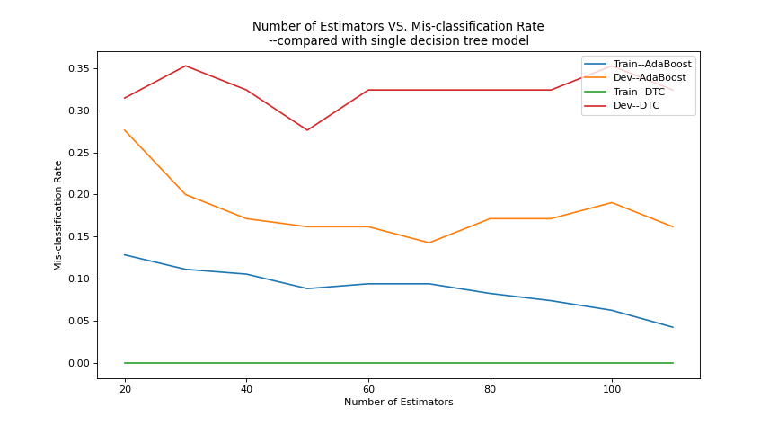
plt.title("Number of Estimators VS. Mis-classification Rate\n" +
"--compared with single decision tree model")
plt.plot(numbers, error_rates, label="Train--AdaBoost")
plt.plot(numbers, error_rates_dev, label="Dev--AdaBoost")
plt.plot(numbers, dtc_error_rates, label="Train--DTC")
plt.plot(numbers, dtc_error_rates_dev, label="Dev--DTC")
plt.xlabel('Number of Estimators'); plt.ylabel('Mis-classification Rate')
plt.legend(loc='upper right')
plt.show()
''' 结果显示:
1.boosting模型测试集错误率明显低于弱分类器dtc;但是
2.模型数量越大训练集误差越小,但是测试集误差只能有限减小,最后震荡在一个范围。
'''
(3)梯度提升
- 提升法:用一种渐进的,阶段改良的方式,从一系列若分类器适配出一个增强模型。具体就是通过错误率调整实例的权重,在下一模型改进不足之处。
- 梯度提升法就是采用梯度而不是权重来鉴别缺陷。以下是一个简单回归问题的梯度提升步骤。
- 给定预测变量 $X$ 和响应变量 $Y$:$X = [x_1, x_2, …, x_N]\ and\ Y = [y_1, y_2, …, y_N]$
- 先从简单模型开始,例如直接使用均值预测所有值:$\hat{y_i} = \sum_i^N(y_i) / N$
- 得到残差:$R_i = y_i - \hat{y_i}$
- 下一个分类在以下数据上训练:$[(x_1, R_1), (x_2, R_2), …, (x_N, R_N)]$
- 进行迭代达到所需准确率
- 为何叫做梯度提升:$F(x_i) - y_i$ 就代表梯度,即该点的一阶导数,正好是负的残差;亦即在简单回归问题中,梯度提升等同于残差缩减
- 梯度提升是一种框架而不仅仅是一种具体的算法,任何可微函数都可以应用到框架中
1
2
3
4
5
6
7
8
9
10
11
12
13
14
15
16
17
18
19
20
21
22
23
24
25
26
27
28
29
30
31
32
33
34
35
36
37
38
39
40
41
42
43
44
45
46
47
48
49
from sklearn.datasets import load_boston
from sklearn.metrics import mean_squared_error
from sklearn.model_selection import train_test_split
from sklearn.preprocessing import PolynomialFeatures
from sklearn.ensemble import GradientBoostingRegressor

def view_model(model):
    print("\nTraining Scores: \n" + '='*66)
    for i, score in enumerate(model.train_score_):
        print(f"Estimator_{i+1:d} Score:\t{score:0.3f}")
    print("\nFeature Importance: \n" + '='*66)
    for i, score in enumerate(model.feature_importances_):
        print(f"Feature_{i+1} Importance:\t{score:0.3f}")
    plt.figure(figsize=(6, 6.75), dpi=80)
    plt.plot(range(1, model.estimators_.shape[0]+1), model.train_score_)
    plt.xlabel("Model Sequence"); plt.ylabel("Model Score")
    plt.show()

# load boston dataset
X, y = load_boston()['data'], load_boston()['target']
# split dataset
x_train, x_temp, y_train, y_temp = \
            train_test_split(X, y, test_size=0.3, random_state=1)
x_dev, x_test, y_dev, y_test = \
            train_test_split(x_temp, y_temp, test_size=0.3, random_state=1)

# generate polynomial features
polyfeat = PolynomialFeatures(2, interaction_only=True)
polyfeat.fit(x_train)
for name in ['train', 'dev', 'test']:
    exec(f"x_{name}_poly = polyfeat.transform(x_{name})")

# build gradient boosting model and report
poly_gbr = GradientBoostingRegressor(n_estimators=500, verbose=10,
            subsample=0.7, learning_rate=0.15, max_depth=3, random_state=1)
# 当verbose>1,将每个模型或树构建时的进展情况打印出来;
# 采样率subsample指定模型采样70%的训练集数据;
# 学习率learning_rate,是一个缩减参数,控制每个模型的贡献;

poly_gbr.fit(x_train_poly, y_train)
y_pred = poly_gbr.predict(x_train_poly)
print("\nModel Performance in Training Set: \n" + '='*66)
view_model(poly_gbr)
print("\nMSE:\t{:0.2f}".format(mean_squared_error(y_train, y_pred)))

# 在验证集上测试结果
y_dev_pred = poly_gbr.predict(x_dev_poly)
print("\nModel Performance in Dev Set: \n" + '='*66)
print("\nMSE:\t{:0.2f}".format(mean_squared_error(y_dev, y_dev_pred)))
第九章 生长树
上述基于树算法具备对抗噪声的健壮性和解决各类问题的广泛能力,能在没有数据整理的情况下获得很好的结果,可作为黑箱工具。
主要优点:挂袋法有天然的并行性;决策树算法在每一层将数据划分,实现隐式的特征选择;几乎不需要对数据进行预处理,不同度量、缺失值或者异常值,以及非线性问题等,对其几乎没有影响。
主要难题:为了避免过拟合进行剪枝的难度;大型树容易导致低偏差和高方差。
(1)随机森林
- 随机森林也是一种挂袋法,基本思路是利用大量的噪声评估器,用平均法处理噪声,以减小最终结果的方差。
- 随机森林构建的是相互之间没有关联的树。具体方法是,在进行结点划分时,不选择所有的属性,而是随机选择一个属性子集。
- 构建随机森林:$LOOP\ for\ 1\ to\ T$
- 随机选择 $m$ 个属性
- 采用预定义的 $criterion$,选择一个最佳属性作为划分变量
- 将数据集划分为两个部分
- 返回划分的数据集,分别在两个部分迭代上述过程
- 最终获得 $T$ 棵树
- 提升法使用弱分类器进行强化,实现较低的方差(较高的验证集准确率);而在随机森林中,构建最大深度的树,但是引入了高方差。随后通过大量树进行投票,解决高方差问题。
1
2
3
4
5
6
7
8
9
10
11
12
13
14
15
16
17
18
19
20
21
22
23
24
25
26
27
28
29
30
31
32
33
34
35
36
37
38
39
40
41
42
43
44
45
46
from operator import itemgetter
from sklearn.datasets import make_classification
from sklearn.metrics import classification_report, accuracy_score
from sklearn.model_selection import train_test_split, RandomizedSearchCV
from sklearn.ensemble import RandomForestClassifier

# generate dataset for classification
X, y = make_classification(n_samples=500, n_features=30, flip_y=0.03,
                           n_informative=18, n_redundant=3, n_repeated=3,
                           random_state=1)
# split dataset
x_train, x_temp, y_train, y_temp = \
            train_test_split(X, y, test_size=0.3, random_state=1)
x_dev, x_test, y_dev, y_test = \
            train_test_split(x_temp, y_temp, test_size=0.3, random_state=1)

# build forest and report
rfc = RandomForestClassifier(n_estimators=100)
rfc.fit(x_train, y_train)
y_pred = rfc.predict(x_train)
y_dev_pred = rfc.predict(x_dev)
train_score = accuracy_score(y_train, y_pred)
dev_score = accuracy_score(y_dev, y_dev_pred)
print(f"Training Accuracy: {train_score:0.2f}\tDev Accuracy: {dev_score:0.2f}")
# 结果方差较大,训练集准确率100%,测试集只有83%

# search parameters
param_dict = {
    "n_estimators": np.random.randint(75, 200, 20),
    "criterion": ['gini', 'entropy'],   #基尼系数与熵判据
    "max_features": [int(np.sqrt(X.shape[1]))*i for i in [1,2,3]] + \
                    [int(np.sqrt(X.shape[1]))+10]   #每个结点选取的特征数
    }
grid = RandomizedSearchCV(estimator=RandomForestClassifier(),
                          param_distributions=param_dict,
                          n_iter=20, random_state=1, n_jobs=-1, cv=5)
grid.fit(X, y)

# view parameters of grid searching
print("\n模型参数:\n" + '='*66)
for score in grid.cv_results_['params']:
    print(score)
print(classification_report(y_dev, grid.predict(x_dev)))
# 当对grid使用predict实例方法时,隐式调用了最优模型
best_model = grid.best_estimator_
print(best_model)
(2)超随机树
- 超随机树(Extra Trees)或称为极限随机树(Extremely Randomized Trees)与随机森林主要有两点不同:
- 不使用自举法,而是使用完整的数据集
- 给定结点随机选择属性数量 $K$,它随机选择割点,不考虑目标变量
- 优势:更好地降低方差,可以在未知数据集上取得很好的效果;并且计算复杂度相对较低
- 构建超随机树:$LOOP\ for\ 1\ to\ T$
- 随机选择 $m$ 个属性
- 随机选取一个属性作为划分变量(忽略任何标准,完全随机)
- … 接下来与随机森林一致
1
2
3
4
5
6
7
8
9
10
11
12
13
14
15
16
17
18
19
20
21
22
23
24
25
26
27
28
29
30
31
32
33
34
35
36
37
38
39
40
41
42
43
44
45
46
47
import numpy as np
from sklearn.datasets import make_classification
from sklearn.metrics import classification_report, accuracy_score
from sklearn.model_selection import train_test_split, cross_val_score
from sklearn.model_selection import RandomizedSearchCV
from sklearn.ensemble import ExtraTreesClassifier

# generate dataset for classification
X, y = make_classification(n_samples=500, n_features=30, flip_y=0.03,
                           n_informative=18, n_redundant=3, n_repeated=3,
                           random_state=1)
# split dataset
x_train, x_temp, y_train, y_temp = \
            train_test_split(X, y, test_size=0.3, random_state=1)
x_dev, x_test, y_dev, y_test = \
            train_test_split(x_temp, y_temp, test_size=0.3, random_state=1)

# build forest and report
etc = ExtraTreesClassifier(n_estimators=100, random_state=1)
etc.fit(x_train, y_train)
y_pred = etc.predict(x_train)
y_dev_pred = etc.predict(x_dev)
print(f"Training Accuracy: {accuracy_score(y_train, y_pred):0.2f}")
print(f"Dev Accuracy: {accuracy_score(y_dev, y_dev_pred):0.2f}")
print("\nCross Validated Score: \n" + '='*66)
print(cross_val_score(etc, x_dev, y_dev, cv=5))

# search parameters (与上一节一样流程,只estimator由随机森林变成extra_trees)
param_dict = {
    "n_estimators": np.random.randint(75, 200, 20),
    "criterion": ['gini', 'entropy'],   #理论来说不需要判断准则
    "max_features": [int(np.sqrt(X.shape[1]))*i for i in [1,2,3]] + \
                    [int(np.sqrt(X.shape[1]))+10]   #每个结点选取的特征数
    }
grid = RandomizedSearchCV(estimator=ExtraTreesClassifier(),
                          param_distributions=param_dict,
                          n_iter=20, random_state=1, n_jobs=-1, cv=5)
grid.fit(X, y)
print("\n模型参数:\n" + '='*66)
for score in grid.cv_results_['params']:
    print(score)
print(classification_report(y_dev, grid.predict(x_dev)))
# 当对grid使用predict实例方法时,隐式调用了最优模型

best_model = grid.best_estimator_
print(best_model)
# 在验证集的准确率达到100%
(3)旋转森林
- 随机森林和挂袋法使用大量的树实现精确的预测,而旋转森林的思路是使用少得的集成数量。
- 构建旋转森林步骤:$LOOP\ for\ 1\ to\ T$
- 将训练集的属性划分为大小相等的 $K$ 个不重叠子集
- 对每个子集,自举 75% 的样本,在样本上执行:
- 在 $K$ 个数据集的第 $i$ 个子集中进行 PCA,保留主成分。对每个特征 $j$, 主成分标为 $a_{ij}$
- 保留以上所有子集的主成分
- 创建 $n*n$ 的旋转矩阵,$n$ 是特征总数
- 将上述的主成分放进旋转矩阵,这些成分匹配特征在初始训练数据集中的位置
- 通过矩阵乘法将训练集投影到旋转矩阵上
- 用投影的数据构建一颗决策树,并保存树和旋转矩阵
1
2
3
4
5
6
7
8
9
10
11
12
13
14
15
16
17
18
19
20
21
22
23
24
25
26
27
28
29
30
31
32
33
34
35
36
37
38
39
40
41
42
43
44
45
46
47
48
49
50
51
52
53
54
55
56
57
58
59
60
61
62
63
64
65
66
67
68
69
70
71
72
73
74
75
76
77
78
79
80
81
82
83
84
85
86
87
88
89
90
91
92
93
94
95
96
97
98
"""python 中还没有包含旋转矩阵算法的库(2016-12)需要自己编写"""
import numpy as np
from sklearn.datasets import make_classification
from sklearn.metrics import classification_report
from sklearn.model_selection import train_test_split
from sklearn.decomposition import PCA
from sklearn.tree import DecisionTreeClassifier

# generate dataset for classification
X, y = make_classification(n_samples=500, n_features=50, flip_y=0.03,
                           n_informative=30, n_redundant=5, n_repeated=5,
                           random_state=1)
# split dataset
x_train, x_temp, y_train, y_temp = \
            train_test_split(X, y, test_size=0.3, random_state=1)
x_dev, x_test, y_dev, y_test = \
            train_test_split(x_temp, y_temp, test_size=0.3, random_state=1)

def random_subset(iterable_obj, k):
    '''get random subset from iterable object, using in next function'''
    subsets = []
    iteration = 0
    limit = len(iterable_obj) / k  #先储存limit,iterable_obj的长度会动态变化
    # 洗牌:
    np.random.shuffle(iterable_obj)
    # 获取k个子集:
    while iteration < limit:
        if k <= len(iterable_obj):
            subset = k
        else:
            subset = len(iterable_obj)
        subsets.append(iterable_obj[:subset])
        del iterable_obj[:subset]    #删除该切片,使子集不相交
        iteration += 1
    return subsets

# ========================== 生成旋转森林的主循环 ===========================

T = 25    #树的数量T
K = 5    #特征子集长度K
models = []    #保存每一棵树
r_matrices = []    #保存与树对应的旋转矩阵
feature_subsets = []    #保存随机选取的特征子集

for i in range(T):
    # 训练集自举,随机选取75%的子集:
    x, _, _, _ = train_test_split(x_train, y_train, test_size=0.25)
    # 在数据集上随机选取特征(生成用于选集的index):
    feature_idx = [idx for idx in range(x.shape[1])]
    random_k_subset = random_subset(feature_idx, K)
    feature_subsets.append(random_k_subset)

    # 生成旋转矩阵:
    rotation_matrix = np.zeros((x.shape[1],x.shape[1]), dtype=float)  #初始化
    for subset in random_k_subset:
        # 对每个特征子集执行PCA,并将所有components存放进旋转矩阵的对应位置:
        # 注意到这个循环只填满一个旋转矩阵,因为每一个subset之间是互斥的
        pca = PCA()
        x_subset = x[:, subset]
        pca.fit(x_subset)
        for ii in range(len(pca.components_)):
            for jj in range(len(pca.components_)):
                rotation_matrix[subset[ii],subset[jj]] = pca.components_[ii,jj]
    r_matrices.append(rotation_matrix)

    # 将输入数据投影到旋转矩阵
    x_transformed = x_train.dot(rotation_matrix)
    # 使用转换的数据构建决策树并保存
    dtc = DecisionTreeClassifier()
    dtc.fit(x_transformed, y_train)
    models.append(dtc)

# =========================== 评估旋转森林模型 =============================
def predict_models(x, models=models, r_matrices=r_matrices):
    '''采用全部模型的预测值进行投票产生最终预测'''
    # 获取每个模型的预测值
    y_predictions = []
    for i, model in enumerate(models):
        x_trans = x.dot(r_matrices[i])
        y_pred = model.predict(x_trans)
        y_predictions.append(y_pred)
    # 结合所有模型的预测得出最终预测
    prediction_matrix = np.matrix(y_predictions)
    final_predictions = []
    for i in range(x.shape[0]):
        predictions = np.ravel(prediction_matrix[:,i])    #降维,扁平化
        nonzero_idx = np.nonzero(predictions)[0]    #返回非零的坐标(元组里面)
        is_one = len(nonzero_idx) > len(models)/2    #投票,过半数为1则返回True
        final_predictions.append(is_one)
    return np.array(final_predictions)

# 分别在训练集和验证集上评估
y_pred = predict_models(x_train)
y_dev_pred = predict_models(x_dev)
print(classification_report(y_train, y_pred))
print(classification_report(y_dev, y_dev_pred))

# 跑了几次,发现效果不好,方差较大。
第十章 大规模机器学习 – 在线学习
本章的关注点是大规模机器学习以及适合处理大规模问题的算法。前几章的所有模型的数据集都是可以完全加载进计算机的内存的。当数据集数目庞大,需要构建一个框架,可以根据部分数据进行判断,并随着新数据的输入而持续提高。
随机梯度下降(Stochastic Gradient Descent)就是一个这样的框架。许多线性方法,如逻辑斯蒂回归、线性回归、线性 SVM,以及非线性的核方法等都可用于 SGD 框架。
(1)用感知器作为在线学习算法
- 感知器(Perceptron):处理大规模学习问题,建模时一次只使用数据集的一部分
- 具体算法:
- 将模型权重用一个小的随机数初始化
- 用输入数据 $X$ 的均值进行去中心化
- 在每个步骤 $t$ 中(或称为纪元):
- 随机选择记录中的一个实例进行预测
- 比较预测标签和真实标签的误差
- 如果预测错误则更新权重
- 如何更新权重?
- 假定在一个纪元中,输入 X 为:$X_i = [x_1, x_2, …, x_m],\ i=1, 2, …, n$
- Y 的集合为:$Y = [1, -1]$
- 则权重定义为:$W = [w_1, w_2, …, w_m]$
- 每条记录得出的预测值为:$\hat{y_i} = sign(w_i * x_i)$
- 权重的更新公式为:$w_t + 1 = w_t + y_i * x_i$
- 增加学习速率参数 $\alpha$:$w_t + 1 = w_t + \alpha * y_i * x_i$
- $\alpha$ 取值一般为 $[0.1, 0.4]$
1
2
3
4
5
6
7
8
9
10
11
12
13
14
15
16
17
18
19
20
21
22
23
24
25
26
27
28
29
30
31
32
33
34
35
36
37
38
39
40
41
42
43
44
45
46
47
48
49
50
51
52
53
54
55
56
57
58
59
import numpy as np
from sklearn.datasets import make_classification
from sklearn.metrics import classification_report
from sklearn.preprocessing import scale, PolynomialFeatures

def get_data(batch_size, kernel='linear'):
    '''生成多组数据模拟大型数据和数据流,隐式返回一个生成器generator'''
    b_size = 0
    while b_size < batch_size:
        X, y = make_classification(n_samples=1000, n_features=30, flip_y=0.03,
                                   n_informative=24, n_redundant=3,n_repeated=3,
                                   random_state=1)
        # 添加非线性核选项:
        if kernel == 'linear':
            X = scale(X, with_mean=True, with_std=True)    #特征数据中心化
        elif kernel == 'polynomial':
            polyfeat = PolynomialFeatures(degree=2)
            X = polyfeat.fit_transform(X)
        y[y<1] = -1    #把y标签由{0, 1}改为{-1, +1}
        b_size += 1
        yield X, y

def build_perceptron(x, y, weights, epochs, alpha=0.5):
    ''' 构建一个感知器模型,用于对于多组数据进行循环建模,模拟现实的数据流。
        weights: 初始权重矩阵;
        epochs: 纪元数,即更新权重的次数;
        alpha: 学习速率。
    '''
    for i in range(epochs):
        # 搅乱数据集:
        shuffled_idx = [i for i in range(len(y))]
        np.random.shuffle(shuffled_idx)    #这个函数是就地更改的
        x_train = x[shuffled_idx, :].reshape(x.shape)
        y_train = np.ravel(y[shuffled_idx])

        # 一次构建一个实例的权重:
        for idx in range(len(y)):
            prediction = np.sign(np.sum(x_train[idx,:] * weights))
            if prediction != y_train[idx]:
                weights = weights + alpha * (y_train[idx] * x_train[idx, :])
    # 所有纪元更新完之后返回权重
    return weights

# 生成 10 组数据流
data = get_data(10, 'linear')    #data = get_data(10, 'polynomial')
# 使用生成器的__next__()方法获取下一组数据
X, y = data.__next__()

# 初始化权重矩阵
weights = np.zeros(X.shape[1])

# 模拟收到10组数据集,进行建模学习
for i in range(10):
    weights = build_perceptron(X, y, weights, 100, 0.5)
    y_pred = np.sign(np.sum(X * weights, axis=1))
    print('='*66+f"\nModel Performance After Receiving Dataset Batch {i+1}:\n")
    print(classification_report(y, y_pred))
    if i != 9:
        X, y = data.__next__()
(2)用梯度下降解决回归问题
标准的回归结构中,有一系列实例:$X = [x_1, x_2, …, x_n]$, 每个实例有 $m$ 个属性(特征):$x_i = [x_{i1}, x_{i2}, …, x_{im}]$。 回归算法的任务是找到一个 $X$ 到 $Y$ 映射:$Y = F(X)$ ,由一个权重向量来进行参数化: $Y = F(X, W) = X\cdot{W} + b$ ,于是回归问题就变成寻找最优权重的问题。采用损失函数进行优化,对 $n$ 个实例的数据集,全局损失函数形式为:$\frac{1}{n} \sum_i^n{ L\lbrace{f(x_i, w), y_i}\rbrace }$。
随机梯度下降(Stochastic Gradient Descent, SGD)是一种优化技术,可用于最小化损失函数。首先要找出 $L(\cdot)$ 的梯度,也就是损失函数对权重 $w$ 的偏导
和批量梯度下降等其他技术不同,SGD 每次只操作一个实例:
- 对每个纪元 $t$ ,搅乱数据集
- 选择一个实例 $x_i$ 及其对应的响应变量 $y$
- 计算损失函数及其对于 $w$ 的偏导 $\nabla{w}$(倒三角符号,表示矢量求偏导)
- 更新权重值
更新权重值的公式为:
$w_t + 1 = w_t - \nabla{w} L(\hat{y_i}, y_i)$
式中权重和梯度的方向相反,这样迫使权重向量降序排列,以减小目标函数。引入学习率后表示为:
$w_t + 1 = w_t - \eta * (\nabla{w} L(\hat{y_i}, y_i))$
在 SGD 的基础上加上正则化,类似岭回归增加 L2 范数正则项和学习率,权重更新公式表示为:
$w_t + 1 = w_t - \eta * (\nabla{w} L(\hat{y_i}, y_i)) + \alpha * (\nabla{w}R(W))$
1
2
3
4
5
6
7
8
9
10
11
12
13
14
15
16
17
18
19
20
21
22
23
24
25
26
27
28
29
30
31
32
33
34
35
36
37
38
39
40
41
42
43
44
45
46
47
from sklearn.datasets import make_regression
from sklearn.model_selection import train_test_split
from sklearn.metrics import mean_absolute_error, mean_squared_error
from sklearn.linear_model import SGDRegressor


# generate dataset for regression
X, y = make_regression(n_samples=1000, n_features=30, random_state=1)
# split dataset
x_train, x_temp, y_train, y_temp = \
            train_test_split(X, y, test_size=0.3, random_state=1)
x_dev, x_test, y_dev, y_test = \
            train_test_split(x_temp, y_temp, test_size=0.3, random_state=1)


# 建模 & 预测
sgdr = SGDRegressor(n_iter=10, shuffle=True, loss='squared_loss',
                    learning_rate='constant', eta0=0.01, fit_intercept=True,
                    penalty='none')
# 上述大部分参数是默认的,写出来看一下而已
# learning_rate指定学习速率的类型,eta0指定学习速率的值
# penalty指定缩减类型(Lr缩减),本例无需进行缩减
sgdr.fit(x_train, y_train)
y_pred = sgdr.predict(x_train)
y_dev_pred = sgdr.predict(x_dev)

# 查看模型参数
print(f"\nModel Intercept: {sgdr.intercept_}")
for i, coef in enumerate(sgdr.coef_):
    print(f"Coefficient_{i+1}: {coef:0.3f}")
# 打印训练集和验证的MSE和MAE
print('\nTrain set: ========>>')
print(f"Mean absolute error: {mean_absolute_error(y_train, y_pred):0.2f}")
print(f"Mean squared error: {mean_squared_error(y_train, y_pred):0.2f}")
print('\nDev set: ========>>')
print(f"Mean absolute error: {mean_absolute_error(y_dev, y_dev_pred):0.2f}")
print(f"Mean squared error: {mean_squared_error(y_dev, y_dev_pred):0.2f}")

# 使用 L2 正则化建模:通过penalty参数指定正则项
regularized_sgdr = SGDRegressor(n_iter=10, learning_rate='constant',
                            penalty='l2', alpha=0.01)    #alpha:正则项缩放
regularized_sgdr.fit(x_train, y_train)
# 查看模型参数
print("\nRegularized Model Coefficients: \n" + '='*66)
for i, coef in enumerate(regularized_sgdr.coef_):
    print(f"Coef_{i+1:d}:\t{coef:0.3f}")
print(f"Model Intercept:\t{regularized_sgdr.intercept_}")
(3)用梯度下降解决分类问题
分类问题除响应变量不同,其他结构与回归问题类似。由于响应变量的性质,需要不一样的损失函数。对于二分类问题,应用逻辑斯蒂回归函数获取预测值:
$F(w, x_i) = 1 / (1 + e^{-x_i * w^T})$
上式被称为 $sigmoid$ 函数。当 $x_i$ 为很大的正数,函数值趋向 1,反之趋向 0。于是可以定义如下的 $log$ 损失函数:
$L(w, x_i) = -y_i * log(F(w, x_i)) - (1-y_i) * log(1 - F(w, x_i))$
将上式代入 SGD 的权重更新公式,即得到分类问题的 SGD。
1
2
3
4
5
6
7
8
9
10
11
12
13
14
15
16
17
18
19
20
21
22
23
24
25
26
27
28
import numpy as np
from sklearn.datasets import make_classification
from sklearn.model_selection import train_test_split
from sklearn.metrics import accuracy_score
from sklearn.linear_model import SGDClassifier


# generate dataset for classification
X, y = make_classification(n_samples=1000, n_features=30, flip_y=0.03,
                           n_informative=18, n_redundant=3, n_repeated=3,
                           random_state=1)
# split dataset
x_train, x_temp, y_train, y_temp = \
            train_test_split(X, y, test_size=0.3, random_state=1)
x_dev, x_test, y_dev, y_test = \
            train_test_split(x_temp, y_temp, test_size=0.3, random_state=1)


# build model and predict
sgdc = SGDClassifier(n_iter=50, loss='log',    #使用log损失函数
                     learning_rate='constant', eta0=1e-4, penalty='none')
sgdc.fit(x_train, y_train)
y_pred = sgdc.predict(x_train)
y_dev_pred = sgdc.predict(x_dev)

# evaluate model and show score
print("Training Accuracy: {0:0.2f}\tDev Accuracy: {1:0.2f}".format(\
        accuracy_score(y_train, y_pred), accuracy_score(y_dev, y_dev_pred)))
END